
60°C Rise Makes 144 MPa Thermal Stress, Unit Aware Checks for Engineers

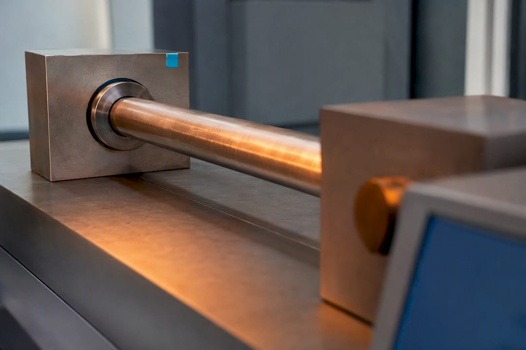
For a fully restrained, linear-elastic isotropic member, thermal stress is σ = E · α · ΔT, and the sign follows directly from the physics: heating a constrained part builds compressive stress, cooling it builds tensile stress. This applies once the member cannot expand or contract freely, strains stay small, and the material behaves elastically across the temperature range in question.
TL;DR:
Ensure all material properties, such as Young’s modulus and the coefficient of thermal expansion, are in matching units before calculating stress.
Recognize that the maximum thermal stress occurs under full restraint; partial restraint reduces the actual stress proportionally to restraint stiffness.
Be cautious of uneven heating; fast temperature gradients can produce localized stresses that exceed steady-state calculations due to internal restraint effects.
Use hand calculations to establish a conservative stress bound before moving to complex finite element analysis for non-uniform or transient thermal conditions.
Confirm your calculations against material yield strengths with appropriate safety factors, especially when approaching the elastic limit.
Table of Contents
How Do You Calculate Thermal Stress From E, α, and ΔT?
Each term in σ = E · α · ΔT carries its own unit conventions, and mixing them up is the single most common source of a wrong answer.
Young’s modulus (E) measures stiffness, usually given in gigapascals (GPa) or megapascals (MPa) in SI work, and pounds per square inch (psi) in imperial calculations. Steel runs around 200 GPa, aluminum closer to 69 GPa. E is not fixed.
Coefficient of linear thermal expansion (α) describes how much a material grows per degree, typically listed as ×10^-6 per °C or per °F. Steel sits near 12×10^-6/°C, while aluminum expands almost twice as fast. Values come from Young’s modulus and thermal expansion references, but always confirm you’re reading the linear coefficient, not the volumetric one.
Temperature change (ΔT) is simply final temperature minus initial temperature (ΔT = Tf − Ti). Get the sign wrong here and every downstream number flips.
A few limitations matter before you trust the output:
The formula assumes an isotropic material with the same properties in every direction.
It assumes small strains and purely elastic behavior, no yielding.
It’s a conservative simplification. Real geometry, partial restraint, or nonlinear material response can push actual stress lower, or in localized spots, higher.
Worked Examples: Steel in SI and Imperial Units
The cleanest way to trust the formula is to run it twice: once in SI, once in imperial, and confirm both land on the same physical answer.
Example 1: SI units, steel bar, fully restrained.
Initial temperature Ti = 20°C, final temperature Tf = 80°C, so ΔT = 60°C.
Material properties: E = 200 GPa, α = 12×10^-6/°C.
Apply the formula: σ = E · α · ΔT = 200,000 MPa × 12×10^-6/°C × 60°C.
σ = 144 MPa (compressive, since the bar is heating).
That 144 MPa is worth pausing on. Structural steel typically yields around 250 MPa, so this fully restrained heating case already consumes more than half the material’s elastic capacity before any external mechanical load is applied at all.
Example 2: Imperial units, same bar, converted properly.
Convert E: 200 GPa ≈ 29,000,000 psi.
Convert α: 12×10^-6/°C ≈ 6.67×10^-6/°F.
Convert ΔT: 60°C change equals 108°F change (since a Celsius-degree interval is 1.8 times a Fahrenheit-degree interval).
σ = 29,000,000 psi × 6.67×10^-6/°F × 108°F ≈ 20,900 psi, which converts back to roughly 144 MPa, confirming the SI result.
Example 3: Restraining force when area is known. If that bar has a cross-sectional area of 500 mm², the axial force follows F = σ · A: F = 144 MPa × 500 mm² = 72,000 N, or 72 kN. In imperial terms, with A = 0.775 in², F = 20,900 psi × 0.775 in² ≈ 16,200 lbf.
The pitfalls that trip people up are almost always unit mismatches, mixing GPa with psi, or forgetting that a Celsius-degree ΔT is not numerically the same as a Fahrenheit-degree ΔT even though the temperatures themselves convert differently. Double-check every unit before you multiply, not after.
Why Does Restraint Matter More Than the Formula Itself?
Free expansion produces zero stress, no matter how large ΔT is. A rod heated in open air simply grows longer and stays stress-free. Stress only appears once something stops that movement.
Constrained expansion produces the full σ = EαΔT result, but real structures rarely sit at either extreme. Partial restraint is the more common case: only the strain that is actually prevented generates stress, so the result scales with how stiff the restraint is relative to the member itself. A bolted flange with some flexibility in the surrounding structure will see less stress than a bar welded rigidly at both ends.
Fully restrained: stress equals EαΔT regardless of the member’s length, since length cancels out of the stress equation.
Partially restrained: effective stress is some fraction of EαΔT, set by relative stiffness between the member and its supports.
Free expansion: zero stress, but length now matters enormously for clearance, joint design, and expansion-gap sizing.
Pro Tip: If you’re unsure how rigid a support really is, run the fully restrained case first as a worst-case bound, then check whether your actual design includes expansion joints, slotted connections, or flexible supports that would justify a lower number. When restraint stiffness, multiple load paths, or anchor behavior get complicated, that’s the signal to move from a hand calculation into a full structural model.
What Happens When Heating Is Uneven or Sudden?
A uniform ΔT applied across a whole part is the easy case. Real components often heat unevenly, and that’s where the simple formula quietly stops being accurate.
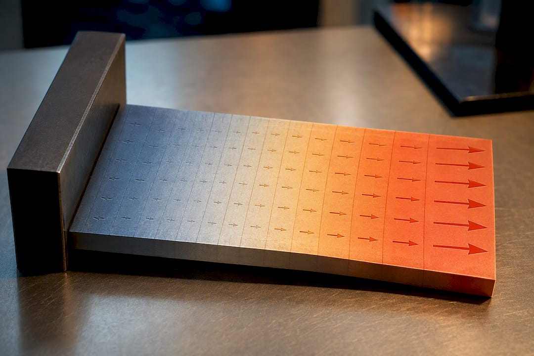
A gradient means the surface of a part changes temperature faster than its interior. Because the two regions want to expand at different rates but are physically connected, they create their own internal restraint, generating localized stress that has nothing to do with the average ΔT of the part.
Thermal shock is the sharpest version of this problem. Rapid heating or cooling drives large surface-to-interior differentials in a short time window, producing tensile stresses at the surface that can exceed the material’s strength even when the bulk temperature change looks modest on paper.
Brittle materials, glass, ceramics, and some cast irons, are especially vulnerable because they have little capacity to yield before cracking.
A practical check: if a part experiences fast temperature transients (quenching, thermal cycling, sudden fluid contact), don’t rely on a steady-state ΔT number alone.
Coupling transient heat conduction with structural finite element analysis (FEA) becomes necessary once gradients, not just averages, drive the failure mode.
When Should You Move From a Calculator to Coupled FEA?
A quick calculator is the right first move for almost every thermal stress question. It handles uniform ΔT cases with known α and E cleanly, and it’s built for conservative hand-checks, including unit conversions and restraining-force calculations when you supply the cross-sectional area.
Escalate to coupled thermal-structural FEA once you’re dealing with transient loading, real temperature gradients, complex or partial restraints, or geometry that creates stress concentrations, sharp corners, holes, thickness transitions, that a single-point hand calculation can’t capture. FE workflows map temperature results onto a structural mesh, and that mapping step needs its own verification: check mesh alignment and tolerance settings before trusting the stress contours that come out.
Step 1: verify your inputs, E, α, ΔT, and units, against a materials reference.
Step 2: run the hand calculator for a conservative bound.
Step 3: compare that result to yield strength with an appropriate safety factor.
Step 4: if the geometry or loading is complex, build a coupled FE model.
A downloadable toolkit fits into that fourth step, offering simulation templates built around conduction, convection, and radiation for readers who need to go past the hand-check stage.
Stage | Tool | Best for |
Hand-check | Calculator (σ = EαΔT) | Uniform ΔT, known E and α, quick bound |
Escalation | Coupled thermal-structural FEA | Gradients, transients, complex restraints |
Applied simulation | Jewlz Technologies toolkit | Conduction/convection/radiation, pressure vessel and CFD tasks |
What Are the Most Common Thermal Stress Calculation Mistakes?
Most calculation errors trace back to a handful of repeatable mistakes, not to the formula itself.
Confirm α, E, and ΔT are all in matching unit systems before multiplying.
Check whether the material property you’re using was measured at the operating temperature, not just at room temperature.
Compare your computed stress against yield strength using a safety factor, commonly in the 1.5 to 3 range, since hand-calculated results reflect elastic theory only and don’t capture plasticity, fatigue, or creep.
Write down your assumptions and boundary conditions as you go, restraint type, temperature source, material grade, so someone else (or you, six months later) can retrace the logic.
Pro Tip: Keep a one-line note next to every calculation stating which safety factor you applied and why. It takes ten seconds and saves an argument later when a reviewer asks how conservative the number really is.
A Practical Note on Hand Calculations vs. Simulation
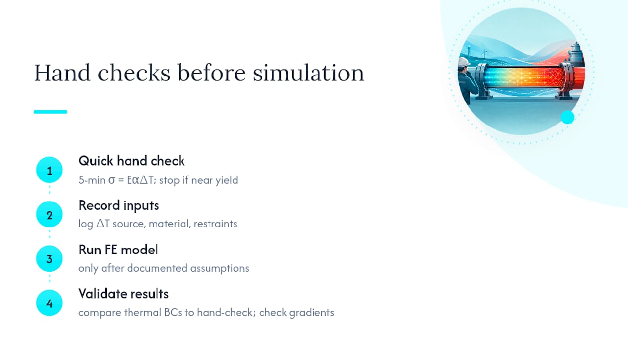
Hand calculations are the gate that keeps expensive simulation time honest. If a five-minute σ = EαΔT check already shows a part near yield, that’s the signal to slow down before committing to a full model, not after.
Good practice means logging every input, ΔT source, material grade, restraint assumption, before touching an FE tool, then validating the thermal boundary conditions against that same hand-check once results come back. When temperature gradients dominate the failure mode rather than a simple average ΔT, that discipline is what keeps a coupled analysis grounded in something checkable.
— Joel
Ready to Move Past Hand Calculations?
A thermal analysis toolkit was built to address the gap this article walks through: the space between a quick σ = EαΔT check and a full coupled thermal-structural model. The toolkit handles conduction, convection, and radiation with a built-in material property database, so you’re not hunting for α and E values across five different datasheets while your ΔT assumptions go stale.

It runs as a downloadable Excel-based tool, which means no new software environment to learn before you get a usable result. If your hand check just flagged a stress that’s uncomfortably close to yield, the next step is trying the thermal analysis toolkit directly, or exploring the broader engineering simulation toolkit if your project also needs pressure vessel or CFD work layered on top. For gradient-heavy problems specifically, the heat conduction reference is worth pairing with it before you build a full transient model.
Where to Verify These Formulas Yourself
For the tensor-level derivation behind σ = E · α · ΔT, MIT OpenCourseWare’s thermoelasticity notes walk through the full structural mechanics treatment. For FE-specific workflow questions, ANSYS’s thermal-stress documentation covers mesh mapping and validation. For quick property lookups and hand-check verification, EngineeringToolBox’s restrained expansion reference is a solid daily-use resource.
Sources
Recommended
Comments