
Thermal Resistance Networks Engineers Build: Example + Templates

Updated: 1 day ago
A thermal resistance network is a 1D circuit model where heat flow plays the role of current and temperature difference plays the role of voltage, letting you calculate steady-state heat transfer through layered materials with simple algebra instead of a full simulation. It works for quick sizing calculations and, when you add thermal capacitance, extends to transient problems like electronics power cycling or wall heat storage. The rest of this guide covers the formulas, the series/parallel rules, the RC transient models, and a full worked example.
TL;DR:
Thermal resistance networks rely on the same series and parallel rules as electrical resistors, but real-world factors like contact resistance and temperature dependence can cause deviations.
In multilayer walls, insulation dominates the temperature drop, but small low-resistance paths like metal studs significantly increase heat flow through the structure.
Transient heat behavior requires adding thermal capacitance at each node, with RC models (Foster and Cauer types) capturing time-dependent response, especially for electronics cooling.
Accurate modeling demands measuring or estimating interface resistances and iterating for temperature-dependent conductivity, as assumptions can lead to underestimating heat transfer.
When network complexity exceeds simple series-parallel, solving a conductance matrix or applying star-delta transforms ensures a precise temperature distribution in more complex geometries.
Table of Contents
How the Electrical Analogy Defines a Thermal Resistance Network
The analogy is exact, not approximate: heat flow $Q$ (watts) behaves like electrical current, and temperature difference $\Delta T$ behaves like voltage. Divide one by the other and you get thermal resistance, $R_{th} = \Delta T / Q$, measured in kelvins per watt (K/W). Low resistance means heat moves easily; high resistance means it’s blocked.
For pure conduction through a flat layer, MIT’s thermodynamics notes define the resistance as:
R = t / (k × A)
where t is thickness, k is thermal conductivity, and A is cross-sectional area. A thicker wall raises resistance linearly. A larger area or a more conductive material lowers it. That single equation is the backbone of every conduction network you’ll ever build.
Convection and radiation get folded into the same framework using an equivalent resistance based on a heat transfer coefficient, h:
Convective resistance: R = 1 / (h × A), where h depends on fluid velocity, geometry, and flow regime.
Radiative resistance: approximated as R = 1 / (h_r × A), where h_r is a linearized radiation coefficient valid over a narrow temperature band.
Combined surface resistance: convection and radiation acting on the same surface combine as parallel resistors, since both paths remove heat simultaneously.
Assembling Networks: Series, Parallel, and Real Engineering Cases
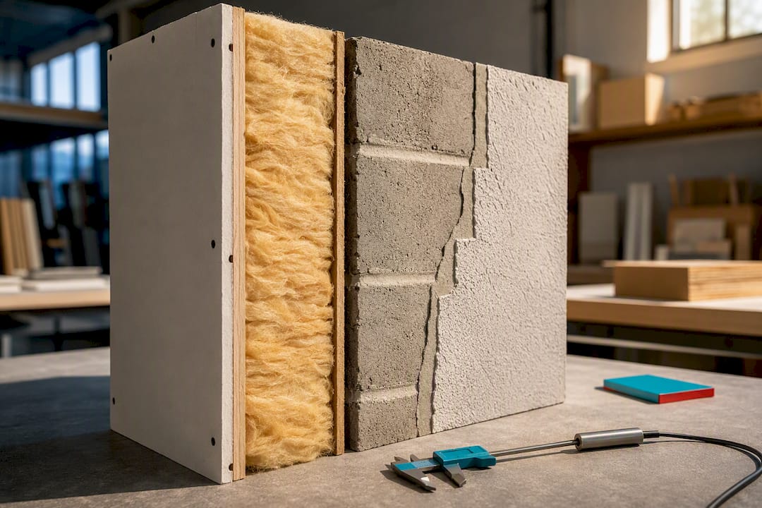
Once you have individual resistances, combining them follows the same rules as electrical resistors. Layers stacked one after another (a wall’s brick, insulation, and drywall) are in series: R_total = R1 + R2 + R3…. Paths that share the same two boundary temperatures but run side by side, like a stud embedded in insulation, are in parallel: 1/R_total = 1/R1 + 1/R2.
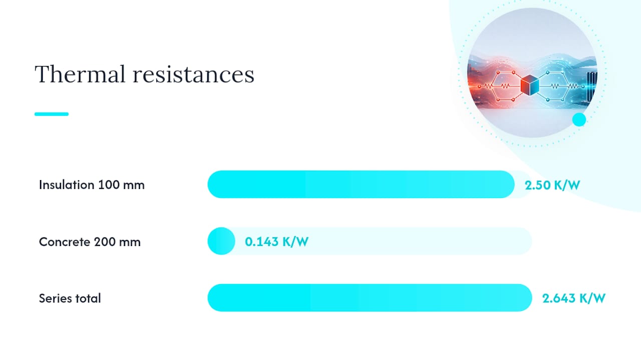
Here’s how that plays out on a real composite slab: 100 mm of insulation (k = 0.04 W/mK) over a 200 mm concrete block (k = 1.4 W/mK), both 1 m² in area, leads to corresponding thermal resistances as calculated by their thickness and conductivity using the formula R = t/(k*A). Total series resistance is the sum of these individual resistances. If the temperature drop across the whole assembly is 20°C, the flux is Q = 20/2.643 ≈ 7.57 W, and you find the interface temperature by multiplying that flux by each layer’s individual resistance.
A thermal bridge changes the math entirely. A steel stud running through insulation creates a parallel path with much lower resistance, so more heat funnels through the metal even though it occupies a small fraction of the wall area. Ignoring that path is one of the most common errors in building thermal calculations.
Practical steps for turning any geometry into a workable network:
Identify the direction of dominant heat flow and collapse the geometry to 1D along that axis.
Split the assembly into layers or parallel branches wherever material properties or geometry change.
Compute each branch’s resistance, then reduce the network stepwise, combining series and parallel groups until you reach a single equivalent R.
Back-substitute to find intermediate node temperatures once the total flux is known.
Don’t. Even a small parallel path with resistance an order of magnitude lower than the surrounding field can dominate the total heat loss.*
How Do Transient RC Thermal Networks Work?
Steady-state resistance networks assume nothing changes with time. Real components heat up gradually, and that behavior needs thermal capacitance, Cth, added at each node. Cth represents a material’s ability to store heat, and paired with resistance it defines a thermal time constant, τ = R × C, the time it takes a temperature step to reach about 63% of its final value.
Two network topologies dominate electronics thermal modeling, and the Nexperia application note on RC thermal models lays out the difference clearly:
Foster networks are curve-fitted to a measured or simulated thermal impedance curve (Zth). They’re mathematically convenient but the individual R and C values don’t correspond to real physical layers.
Cauer networks map each R-C pair to an actual physical layer, junction, package, board, so you can attach an external network (a heatsink or PCB model) at the correct physical node.
Foster models can be converted to Cauer form mathematically, but the conversion isn’t unique without extra physical constraints.
For packaged electronics, JEDEC JESD15-3 formalizes a two-resistor compact model using θJC (junction-to-case) and θJB (junction-to-board). JEDEC recommends using measured resistance values whenever they’re available, falling back to simulated values only when measurement isn’t practical.
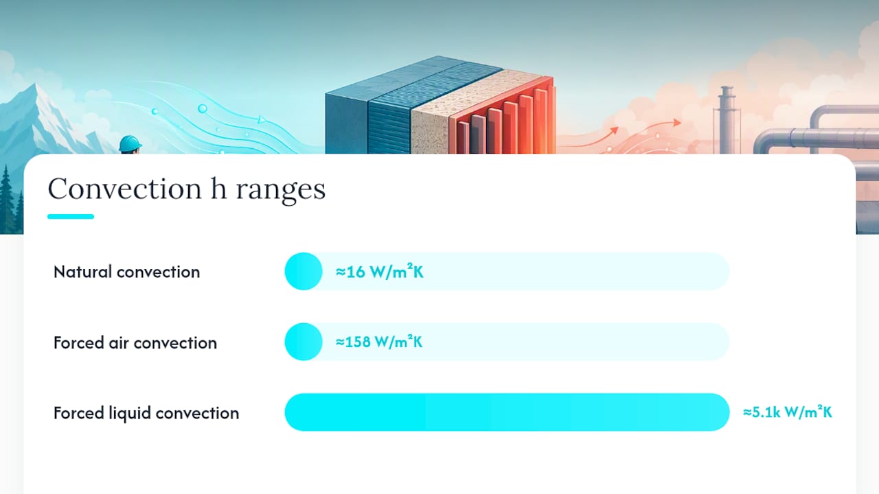
Heat transfer coefficients matter more than most engineers assume. JEDEC’s own guidance lists natural convection around 2 to 30 W/m²K, forced air convection from roughly 15 to 300 W/m²K, and forced liquid convection anywhere from 200 to 10,000 W/m²K, a range spanning three orders of magnitude that can swing your case-to-ambient resistance by a similar factor.
Building these networks in a spreadsheet or a SPICE-like tool is standard practice, and JEDEC explicitly documents spreadsheet and network-calculator workflows as an accepted method for assembling compact models.
When Do Networks Break Down, and What Do You Do Then?
Not every network reduces cleanly to series and parallel combinations. A grid of nodes with cross-connections, like a heat spreader with multiple contact points, needs a full nodal solve. You assemble a conductance matrix G from every branch’s 1/R value, apply known boundary temperatures and any heat source vector Q, then solve G·T = Q for the unknown node temperatures. It’s a linear algebra problem, and it scales to any topology no matter how tangled.
A second trick worth knowing is the Y-Δ (star-delta) transform, borrowed directly from circuit theory, which lets you convert a three-branch star topology into an equivalent triangle (or back), simplifying networks that would otherwise resist direct reduction.
Networks fail to represent reality when:
Heat flow is genuinely three-dimensional and a 1D path can’t capture it, corners, edges, and localized heat spreading are common culprits.
Radiation becomes nonlinear at high temperatures, since it scales with T⁴ rather than ΔT, breaking the simple resistance analogy.
Thermal conductivity varies meaningfully with temperature across the operating range, requiring iterative resistance updates rather than one fixed value.
When any of those apply, a 1D network gives you a fast first estimate, but confirming it with a 3D CFD or FEM simulation is worth the extra time before you commit to a design.
Worked Example: Solving a Multilayer Wall With an Optional PCM Layer
Consider a wall built from four layers, 1 m² of area, indoor air at 22°C and outdoor air at 2°C: 12 mm drywall (k = 0.17 W/mK), 90 mm fiberglass insulation (k = 0.04 W/mK), 100 mm concrete block (k = 1.4 W/mK), and an outer 10 mm stucco finish (k = 0.72 W/mK).
Summed in series, total R = 2.406 K/W. With a temperature difference across the assembly. Heat flux can be estimated by dividing the temperature difference by the total thermal resistance.
Finding the node temperature at each interface is a matter of walking the flux through each layer sequentially:
Start at 22°C on the indoor face.
Subtract Q × R for each layer in order (drywall, then insulation, then concrete, then stucco).
Confirm the final result lands at 2°C on the outdoor face, which checks your arithmetic.
The insulation layer, unsurprisingly, carries almost all of the temperature drop. That’s the point of putting it there.
For transient behavior, add a capacitance node at each layer boundary. Simulations of a thin paraffin PCM layer inserted into a similar wall assembly show it can shift the interior thermal peak from around one hour to roughly 5.5 hours while cutting oscillation amplitude sharply, a useful lever when you’re trying to delay peak cooling load into off-peak hours.
Where Thermal Resistance Networks Break Without These Fixes
Contact resistance at material interfaces is the single most underestimated term in most hand calculations. Two “touching” surfaces almost never make perfect thermal contact, air gaps and surface roughness add real resistance that a pure R = t/(kA) model ignores entirely. Measure it directly when the stakes justify it; otherwise use published interface resistance values rather than assuming zero.
Temperature-dependent conductivity means your first-pass R values are only a starting guess. Recompute k at the average layer temperature, resolve the network, and iterate until node temperatures stop shifting meaningfully between passes, usually two or three iterations for most engineering materials.
Round 3D features (corners, fasteners, embedded conduits) into an equivalent 1D area correction rather than ignoring them.
Cross-check any network result against a quick 3D spot simulation on the geometry that worries you most.
Run a sensitivity study on your least-certain input, often the convective coefficient, before trusting the output.
Pro Tip: If your calculated flux changes by more than a few percent when you nudge k by its expected measurement uncertainty, your model is more sensitive to material data than to geometry, spend your validation effort there first.
Jewlz Technologies Resources for Thermal Resistance Network Analysis
Jewlztech’s Thermalysis Toolkit is a web-based engineering application for analyzing thermal resistance networks using the conduction, convection, and radiation relationships covered above. Engineers can evaluate composite systems and package-level thermal problems using integrated calculations and material properties without building the analysis from a blank spreadsheet. For package-level work, the PCB thermal analysis workflow demonstrates how resistance-network methods can be applied to electronic systems. When greater geometric detail is required, a CFD simulation can provide an additional comparison for identifying three-dimensional effects.
An Editorial Take on Building Thermal Networks That Actually Hold Up
Most guides to thermal resistance treat it as a formula to memorize: R = t/(kA), done. That’s the easy 20% of the problem. The part that separates a usable model from a wrong one is everything this article spent the most space on, contact resistance, temperature-dependent properties, and knowing when a bridge or a 3D corner is about to wreck your series-parallel assumption.
The conventional advice to “just build the network and solve it” undersells how much judgment goes into deciding what counts as a node in the first place. JEDEC’s own recommendation to prefer measured resistance values over simulated ones is a quiet admission that even a well-built compact model is an approximation waiting to be corrected by real data.
If you take one thing from this guide, prioritize verification over elegance. A network model you’ve cross-checked with a single 3D spot simulation is worth more than a beautifully reduced circuit you’ve never tested against reality. Build the network first, because it’s fast and it teaches you where the resistance actually lives. Then spend your remaining time finding out where it’s wrong.
— Joel
Sources
Recommended
Comments