
How to Calculate Thermal Expansion: Formulas and Worked Examples

ΔL = α·L₀·ΔT is the formula, and L = L₀(1 + αΔT) gives you the final length. That’s the entire thermal expansion calculation in one line. For area, use ΔA ≈ 2α·A₀·ΔT, and for volume, ΔV ≈ 3α·V₀·ΔT, where the volumetric coefficient β ≈ 3α for isotropic solids.
Here’s a number to anchor it: a 1-meter steel rod with α ≈ 12×10⁻⁶/°C, heated through a 50°C rise, expands by ΔL = 0.0006 m, or 0.6 mm. That’s roughly the thickness of a credit card, stretched out from a rod you could span with your arms.
α is expressed in 1/°C or 1/K (they’re numerically equivalent for temperature differences)
ΔT can be in Celsius or Kelvin without conversion, since a one-degree change is identical on both scales
Small ΔL numbers compound fast across long spans or large volumes, which is why bridges, pipelines, and tanks all need this math before anything else
Key Takeaways
Thermal expansion calculation starts with ΔL = α·L₀·ΔT, but accurate engineering results depend on matching the right coefficient, temperature range, and restraint condition to that formula.
Point | Details |
Core formula | ΔL = α·L₀·ΔT gives length change; L = L₀(1 + αΔT) gives final length. |
Volume shortcut has limits | ΔV ≈ 3α·V₀·ΔT only holds for isotropic materials, not composites or crystals. |
Coefficients vary by material | Steel (≈12×10⁻⁶/°C) differs enough to matter in mixed-material designs. |
Restraint changes everything | A constrained member develops stress (σ ≈ E·α·ΔT) instead of simply expanding freely. |
Escalate when it gets complex | For coupled, composite, or large-ΔT problems, Jewlztech’s thermal and CFD simulation tools go beyond hand calculations. |
Table of Contents
Thermal Expansion Formula: Variables, Units, and Rearrangements
Coefficient of Thermal Expansion: Reference Table for Common Materials
Using a Thermal Expansion Calculator Without Making Costly Mistakes
Accuracy Limits: When the Simple Thermal Expansion Formula Breaks Down
Free Expansion vs. Constrained Members: Estimating Thermal Stress
Selecting the Right Coefficient for Composites and Engineered Materials
Phase Changes and Their Effect on Thermal Expansion Behavior
Thermal Expansion Formula: Variables, Units, and Rearrangements
Every symbol in the linear thermal expansion formula does specific work. α is the coefficient of thermal expansion, a material property usually given in 1/°C, 1/K, or µm/(m·°C) for small values. L₀ is the original length, ΔT is the temperature change, and ΔL is how much the object grows or shrinks.
The core relationship rearranges cleanly depending on what you’re solving for:
Find the change in length: ΔL = α·L₀·ΔT
Find the final length: L = L₀ + ΔL = L₀(1 + αΔT)
Find the coefficient from test data: α = ΔL / (L₀·ΔT)
Find the required temperature change: ΔT = ΔL / (α·L₀)
Celsius and Kelvin differences are interchangeable in these formulas, since both scales use the same-size degree. Fahrenheit is not. Convert first using °C = (°F − 32) / 1.8, and make sure your α value is already in 1/°C, not 1/°F, before you plug in.
For volume, use ΔV = β·V₀·ΔT directly when a supplier gives you β (common for liquids and gases). For solids where you only have α, the shortcut β ≈ 3α works fine, but only for isotropic materials, a caveat that matters more than most calculators let on.

Coefficient of Thermal Expansion: Reference Table for Common Materials
You don’t need a materials database for most design checks. You need a handful of trustworthy α values and the sense to know when they stop being trustworthy. The table below lists typical linear coefficients near room temperature, drawn from standard physics references.

Invar exists specifically because engineers needed something that barely expands, which is why it shows up in precision instruments and reference standards. Water’s volumetric β dwarfs any solid’s linear α, one reason contained liquids in rigid tanks demand careful volume checks.
Pro Tip: α isn’t a fixed constant across all temperatures. For a large ΔT, pull an average α over your specific range from a manufacturer table rather than using the single 20°C value listed here.
Worked Thermal Expansion Examples for Engineering Design
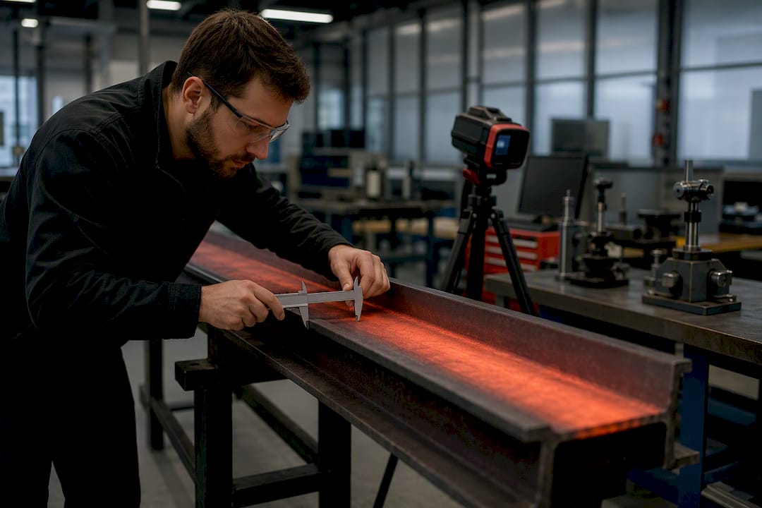
Example 1: Steel I-beam in a structure. A 10-meter carbon steel beam (α = 12×10⁻⁶/°C) sits through a seasonal swing of 60°C.
ΔL = (12×10⁻⁶) × 10 × 60 = 0.0072 m, or 7.2 mm
Final length: L = 10 + 0.0072 = 10.0072 m. That 7.2 mm has to go somewhere, which is exactly why steel-framed buildings use slip joints and roller supports instead of bolting everything rigid.
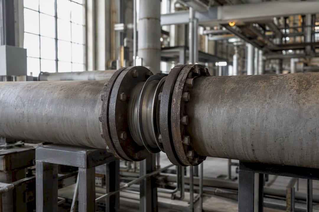
Example 2: Pipe run expansion gap. A 30-meter carbon steel pipe run experiences a 100°C temperature rise during startup.
ΔL = (12×10⁻⁶) × 30 × 100 = 0.036 m, or 36 mm
That’s over an inch of growth. Compare it against a typical expansion joint gap, often designed for 25 to 50 mm of travel depending on the piping code, and you can see immediately whether the planned joint spacing is adequate or whether you need an expansion loop.
Example 3: Volumetric check on a steel tank filled with gasoline. A rigid steel tank holds 10 m³ of gasoline (β ≈ 950×10⁻⁶/°C) and warms by 20°C. Using ΔV = β·V₀·ΔT:
ΔV = 950×10⁻⁶ × 10 × 20 = 0.19 m³, or about 190 liters
The steel shell itself grows too (using 3α), but at roughly 7×10⁻⁶ per degree effective, it’s negligible next to the liquid’s expansion. That mismatch is precisely why sealed tanks need vent capacity or ullage space, not just a strong shell. Every example here assumes a constant average α or β across the range. That’s a reasonable simplification for a 20 to 100°C swing, less so for cryogenic or furnace-level extremes.
Using a Thermal Expansion Calculator Without Making Costly Mistakes
A calculator is only as good as what you feed it. Before trusting an output, confirm four things: the geometry mode (linear, area, or volume), the correct α or β for your exact material, ΔT in consistent units, and whether the tool assumes unrestrained free expansion, which most do by default.
That last assumption trips up more people than bad coefficients. A practical calculator computing free-expansion ΔL tells you nothing about the stress that builds up if the part is bolted down at both ends. Other recurring mistakes:
Applying the 3α shortcut to a value that’s already a volumetric β, effectively tripling an already-correct number
Mixing a °F-based ΔT with an α value defined in 1/°C
Ignoring restraints and treating every joint as if it moves freely
Using a single α across a 500°C range where the real coefficient shifts noticeably
For coupled problems, temperature gradients across a part, thermal expansion interacting with fluid flow, or pressure vessel behavior under thermal cycling, hand calculations stop being reliable. That’s when it’s worth stepping up to full simulation using Jewlztech’s thermal analysis toolkit, which handles variable material properties and multiple heat transfer modes in one model instead of a chain of manual approximations.
Accuracy Limits: When the Simple Thermal Expansion Formula Breaks Down
The linear approximation assumes α stays constant. It doesn’t, not exactly. α creeps upward with temperature for most metals, so a single coefficient pulled from a room-temperature table quietly loses accuracy as ΔT grows.
For ranges under roughly 100°C, a single average α is usually fine for engineering purposes
For larger swings, pull α(T) from a manufacturer curve and use the average across your actual operating range
For extreme ranges (furnace, cryogenic, aerospace reentry), integrate α(T) numerically or break the range into smaller subintervals with local α values
Anisotropy is the other trap. Wood, composites, and many crystals expand differently along different axes, so the tidy β ≈ 3α shortcut simply doesn’t apply. A carbon-fiber panel might barely grow along the fiber direction while expanding several times more across it. Treating it as isotropic with one scalar coefficient will hand you a wrong number with total confidence.
Pro Tip: For anything safety-critical, validate your calculated ΔL against supplier data or a physical measurement before locking in tolerances. A five-minute cross-check beats a field failure.
Free Expansion vs. Constrained Members: Estimating Thermal Stress
Free expansion is the easy case: nothing stops the part from growing, so ΔL happens and that’s the end of the story. Real structures rarely offer that luxury. Pipe runs get anchored, beams get bolted, and slabs get poured against adjacent slabs. When expansion is blocked, the material pushes back, and that pushback shows up as internal stress instead of movement.
For a fully restrained member, the standard screening estimate is:
σ ≈ E·α·ΔT, where E is the material’s Young’s modulus
For steel: E ≈ 200 GPa, α ≈ 12×10⁻⁶/°C, ΔT = 60°C
σ ≈ 200×10⁹ × 12×10⁻⁶ × 60 = 144 MPa
That’s a meaningful fraction of mild steel’s yield strength (roughly 250 MPa), from thermal loading alone, with zero mechanical load added on top. It’s exactly why expansion joints, sliding supports, and pipe loops exist: they convert a stress problem back into a displacement problem, which is far cheaper to manage.
Treat σ ≈ EαΔT as a screening number only. It ignores friction at supports, local stress concentrations at welds or fittings, and buckling risk in slender restrained members, all of which a full structural or FEA analysis will catch and a hand calculation won’t. Anchor loads from restrained thermal growth have buckled pipe racks and cracked foundations; the formula is a warning light, not a verdict.
Jewlz Technologies: Tools Built for Deeper Thermal Analysis
Hand formulas get you a fast answer. When a design involves coupled heat transfer, non-uniform temperature fields, or pressure vessel behavior under thermal load, Jewlztech’s free engineering tools pick up where the calculator leaves off.
Thermal radiation calculations for parts heated unevenly by radiative sources
Heat transfer modeling guidance for choosing between hand math and simulation
Heat conduction worked examples for temperature gradients through solids
PCB thermal analysis for dimensional stability in electronics assemblies
These resources extend the formulas above into the messier conditions real hardware actually experiences.
Selecting the Right Coefficient for Composites and Engineered Materials
A single α value works for a steel rod. It falls apart for a fiberglass panel, a carbon-fiber tube, or a multilayer PCB substrate, because engineered materials rarely expand the same amount in every direction.
Start by checking whether the material is isotropic or directional. Metals, most glasses, and many plastics are close enough to isotropic that one α value and the β ≈ 3α shortcut hold up fine. Composites almost never are. A unidirectional carbon-fiber laminate might show α near zero, or even slightly negative, along the fiber axis, while expanding at rates closer to the resin matrix across it, sometimes 10 to 20 times higher than the axial value.
For these materials, pull coefficients along each relevant axis (longitudinal, transverse, through-thickness) from the manufacturer’s datasheet rather than estimating from a generic materials table. Layered structures, like PCBs, composite panels, or bonded assemblies, need a weighted or laminate-theory approach, since each layer’s coefficient and stiffness both factor into how the whole stack deforms.
When manufacturer data isn’t available, rule-of-mixtures estimates using fiber and matrix volume fractions can get you in the right range, but treat that number as a rough estimate, not a design value. For anything load-bearing or dimensionally critical, either request measured α data from the supplier or run the layup through simulation rather than trusting a hand-calculated approximation.
Accounting for Non-Uniform Temperature Distribution
The ΔL = αL₀ΔT formula assumes one clean, uniform ΔT across the whole part. Real components rarely heat that evenly. A pipe wall exposed to hot fluid on the inside and ambient air outside develops a temperature gradient through its thickness. A large steel plate heated from one edge won’t expand uniformly until the temperature equalizes.
The practical fix for a simple gradient is to break the part into segments, apply local ΔT to each, and sum the resulting ΔL values, effectively treating the calculation as a piecewise integration rather than one global number. For a beam or rod with a linear temperature gradient from one end to the other, using the average temperature change across the length gives a reasonable first-order estimate of total elongation, even though local stress distribution still varies point to point.
Where the gradient is steep or the geometry is complex, a beam that’s hot on one face and cool on the other doesn’t just grow, it bends, since one side expands more than the other. That bending effect (thermal bowing) isn’t captured by the basic linear formula at all and requires either a differential expansion calculation across the cross-section or full thermal-structural simulation. Engineers handling furnace walls, exhaust manifolds, or any component with a strong one-sided heat source should treat the uniform-ΔT formula as a starting estimate, then verify with a temperature-mapped model when the gradient is significant.
Phase Changes and Their Effect on Thermal Expansion Behavior
Thermal expansion formulas assume the material stays in one phase throughout the temperature change. That assumption fails at a phase transition, and the failure isn’t subtle.
Water is the classic case: it expands as it cools toward 4°C, then contracts slightly further as it approaches freezing, before expanding dramatically as it turns to ice. None of that reversal shows up in a simple β·V₀·ΔT calculation, because β itself isn’t constant through the transition. Metals show a milder version of the same problem: many undergo a crystal structure change (an allotropic transformation) at specific temperatures, and α often shifts abruptly at that point rather than following a smooth curve.
For engineering purposes, the practical rule is simple: never extend a single α or β value across a phase boundary. If a design’s operating range crosses a melting point, a crystal transition, or a freeze/thaw cycle, split the calculation into separate segments, one set of coefficients below the transition, another above it, and add the transition’s own volume change (like ice formation) as a separate term rather than folding it into the linear expansion math. Cryogenic systems are particularly exposed to this, since boil-off and phase-change behavior near a liquid’s boiling point can dominate the overall volume response far more than ordinary thermal expansion does.
Building Thermal Expansion Calculations into Design Codes
Engineering codes don’t leave thermal expansion as an afterthought. Structural steel codes require designers to account for thermal movement in expansion joint spacing, and piping codes specify allowable stress limits that explicitly include thermal loading alongside pressure and weight. HVAC and building system guidelines, including ASHRAE’s design guidance, address how ductwork, piping, and structural elements should accommodate seasonal and operational temperature swings without binding or leaking.
The general pattern across codes is consistent: calculate the free-expansion movement first using the basic α·L₀·ΔT relationship, then check that movement against the joint, support, or clearance detail specified for that application. Where full restraint is unavoidable, codes typically require a stress check using material-specific allowable stress values rather than accepting a bare σ ≈ EαΔT screening number as final.
Bringing thermal expansion calculations into a formal design workflow means documenting the α value and its source, the ΔT range assumed (including any seasonal or operational extremes), and whether the check covers free movement, restrained stress, or both. That documentation matters most during code review or failure investigation, when someone needs to trace exactly which assumptions produced a given clearance or stress number. Treating the calculation as a one-time hand check, rather than a documented part of the design basis, is one of the more common gaps auditors find in as-built engineering packages.
What the Formulas Don’t Tell You
The math behind thermal expansion is almost suspiciously simple. Three formulas, a coefficient table, and a calculator will get a student through most homework sets and a working engineer through most first-pass checks. That simplicity is also the trap.
The conventional advice stops at “plug in the numbers.” What actually separates a correct calculation from a costly mistake is knowing which assumption just quietly failed: whether the part is really restrained, whether the material is really isotropic, whether one α value can really cover the whole temperature range. Those aren’t edge cases you’ll stumble into rarely. Anisotropic composites, non-uniform gradients, and large ΔT ranges show up constantly in real design work, far more often than the clean, single-material, uniform-ΔT examples most textbooks use.
If there’s one habit worth building early, it’s treating every thermal expansion number as conditional rather than final. Ask what would break the calculation before trusting it: Is this member actually free to move? Does this α value hold at this temperature? Is this material direction-independent? A five-minute sanity check against those three questions catches more real-world errors than a more precise fourth decimal place ever will. The formula gives you a starting number. The judgment about when that number stops applying is the actual engineering.
Get Thermal Expansion Right the First Time with Jewlztech
Hand calculations tell you how much a part moves. They don’t tell you what happens when that movement runs into a fluid flow problem, a pressure vessel under thermal cycling, or a coupled heat transfer scenario that no single formula captures cleanly. That’s the gap Jewlztech’s toolkit is built to close.

The Thermalysis Toolkit extends the calculations in this article into full conduction, convection, and radiation modeling, with a built-in material property database so you’re not hunting down α values from five different sources. For fluid-coupled problems, the CFD simulation software handles thermal expansion interacting with flow in ways a spreadsheet formula simply can’t. Working with cryogenic storage or large ΔT ranges where phase behavior matters? The cryogenic pressure vessel and boil-off simulator is built specifically for that regime.
Start with the free tools for your next quick check, and when the problem outgrows a hand calculation, move straight into the toolkit without switching platforms or rebuilding your model from scratch.
Sources
Recommended
Comments