
Solver Focused Radiation Modeling in CFD for Engineers: Start with DO

Use Discrete Ordinates (DO) for any participating medium with soot, combustion products, or dense particles. Use Surface-to-Surface (S2S) for clear-air enclosure problems with no absorbing gas. Use P-1 or Rosseland when the medium is optically thick and you need speed over precision. The deciding variable is almost always optical thickness, not personal preference, and solver settings (spectral bands, scattering treatment, wall boundary conditions) determine whether that model choice actually pays off.
TL;DR:
Discrete Ordinates is the preferred model for participating media with soot or dense particles, especially in combustion applications, due to its versatility across optical thickness ranges.
Surface-to-Surface modeling is ideal for clear-air enclosures with no gas absorption, but becomes computationally expensive as surface complexity increases, and is useless if the gas participates in radiation.
Radiation modeling is generally unnecessary below moderate temperatures unless high accuracy in high-temperature environments is required, as convection and conduction dominate heat transfer.
Proper coupling frequency and angular resolution are more critical than the choice of model itself; testing convergence and energy balance is essential to ensure physical accuracy.
Monte Carlo provides the highest accuracy for complex scattering but is costly; use it primarily for validation rather than routine simulations.
Table of Contents
Radiation Modeling CFD: When Do You Actually Need It?
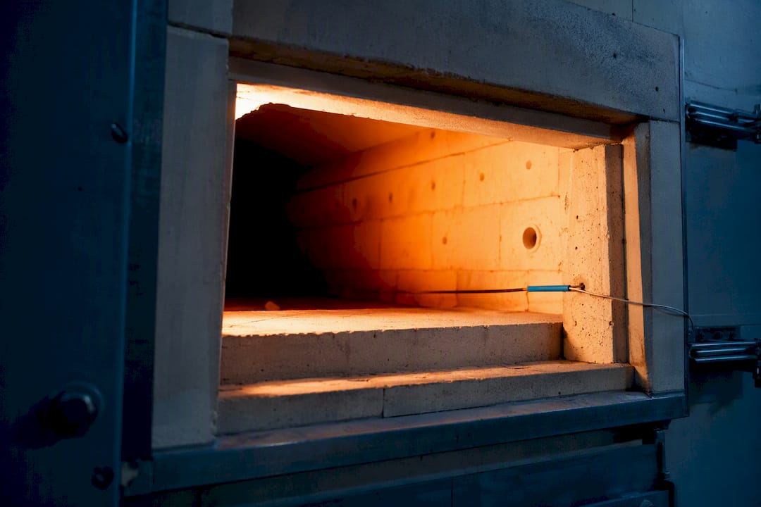
Radiation scales with temperature to the fourth power. Double the absolute temperature of a surface and its radiative emission increases sixteenfold, which is why radiation modeling in CFD becomes unavoidable above moderate temperatures and dominant at high temperatures. Below that range, convection and conduction usually carry the load, and turning on a radiation model just burns compute time for a rounding-error correction.
The practical trigger is optical thickness, defined as the absorption coefficient (a) multiplied by the characteristic path length (L). A low optical thickness means the medium is essentially transparent to radiation, and a surface-based model works fine. A value above 1 means photons are absorbed and re-emitted many times before escaping, which calls for a volumetric or diffusion-based approach. A furnace with soot loading and an average path length in meters might sit in the participating-media regime. A clean HVAC duct with a similar path length may be effectively non-participating.
That distinction, participating versus non-participating media, is the single biggest fork in the road:
Non-participating media: room air, clean combustion products in low-soot burners, most electronics-cooling enclosures. Radiation travels between surfaces with negligible absorption in the gas itself.
Participating media: sooty flames, pulverized coal combustion, dense water droplet sprays, glass melts, and any gas mixture with high CO2 or H2O concentration at high temperature.
Where radiation modeling gets expensive is in the added directional and spectral resolution rather than the base solve. Enabling a volumetric model like DO with modest angular discretization and multiple spectral bands can noticeably increase iteration time, plus meaningfully more memory for storing directional intensities at every cell. Peer-reviewed analysis of CFD radiation modeling confirms that coupling radiation properly to the energy and flow equations, rather than bolting it on as an afterthought, is what determines whether that added cost buys real accuracy.
Which Radiation Model Should You Use? A Quick Comparison
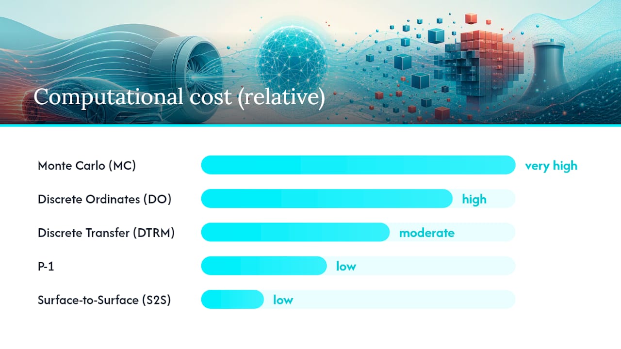
No single model wins across every case, and picking the wrong one either wastes compute or hands you a confidently wrong temperature field. Comparative review literature consistently points to DO and Monte Carlo as the two models capable of representing the full radiative transfer equation across a wide range of optical thickness, with P-1, Rosseland, S2S, and DTRM each trading some of that generality for speed.
Discrete Ordinates (DO) Best for: participating media across nearly any optical thickness, semi-transparent walls, combustion. Pros: handles gray and non-gray spectral treatment, works from optically thin to thick, supports scattering. Cons: angular resolution choices directly affect both accuracy and runtime; coarse discretization creates “ray effect” artifacts.
P-1 Best for: optically thick, highly scattering media like dense particulate flows or glass. Pros: cheap, stable, converges fast, couples easily with the energy equation. Cons: breaks down near boundaries and in optically thin regions; assumes near-isotropic radiation.
Surface-to-Surface (S2S) Best for: enclosure radiation with no participating gas, like electronics housings or building interiors. Pros: no need to resolve radiation through the fluid at all, so it is fast for the right problem. Cons: view-factor calculation and storage get expensive fast as surface count grows; useless once the gas actually absorbs or emits.
Rosseland Best for: extremely optically thick media where the diffusion limit clearly holds. Pros: the cheapest volumetric option, minimal extra memory. Cons: invalid near walls and in anything but very thick media; a poor choice whenever boundary-layer radiative flux matters.
Discrete Transfer (DTRM) Best for: geometries where ray paths can be precomputed once and reused across iterations. Pros: reduces to a manageable set of representative rays, decent for moderate participating media. Cons: no true volumetric scattering, and the ray file needs regenerating whenever geometry changes.
Monte Carlo (MC) Best for: complex scattering, non-gray spectral behavior, and validation-grade accuracy checks. Pros: statistically unbiased, handles nearly any geometry or phase function. Cons: computationally the most expensive; requires enough photon histories to keep statistical noise under control.
Here’s the shortlist that matters in practice: start with DO for anything involving combustion or particulate media, use S2S when the gas itself is transparent, and avoid Rosseland anywhere near a wall you actually care about. Reserve Monte Carlo for cases where you need a trusted benchmark against a faster model, not as your daily driver.
Model | Best for | Accuracy | Computational cost | Key limitation |
DO | Participating media, combustion | High, gray/non-gray | Moderate to high | Angular resolution sensitivity |
P-1 | Optically thick, scattering media | Moderate | Low | Fails near boundaries |
S2S | Clear-air enclosures | High for its scope | Moderate (view factors) | No gas absorption/emission |
Rosseland | Very thick media only | Low outside thick limit | Very low | Invalid near walls |
DTRM | Fixed geometry, moderate media | Moderate | Low to moderate | No volumetric scattering |
MC | Complex scattering, validation | Highest (unbiased) | Highest | Statistical noise, runtime |
How Does the Discrete Ordinates Model Work?
DO divides the full sphere of directions around each cell into a finite set of discrete solid angles and solves a transport equation along each one, approximating the radiative transfer equation without assuming isotropy. Angular resolution is the setting that decides everything: too coarse (say a 2x2 division per octant) and you get “ray effect” streaking where radiation appears to travel in unnatural beams rather than spreading smoothly.

For gray media, one spectral band suffices. For combustion gases with strong wavelength-dependent absorption from CO2 and H2O, switch to a banded (non-gray) treatment with weighted-sum-of-gray-gases or similar spectral models, typically four to seven bands for engineering accuracy.
Watch three solver knobs closely: angular discretization order, radiation-to-flow coupling frequency (solving radiation every iteration is rarely necessary and every 10 to 20 iterations often suffices), and the radiation-specific convergence residual, which should drop independently of the flow residuals before you trust the result.
Pro Tip: Increase angular resolution before you increase spectral bands. A finer angular discretization with one gray band usually beats a coarse angular grid with five spectral bands, at lower total cost.
When Should You Use Diffusion Approximations Like P-1?
P-1 treats radiative intensity as a first-order spherical harmonics expansion, essentially assuming radiation diffuses through the medium the way heat diffuses through a solid. That assumption holds only when the medium is optically thick enough that photons scatter or absorb many times before reaching any boundary. P-1 model documentation puts the practical threshold around an optical thickness of 1 or higher for the approximation to hold reasonably well.
The Rosseland model requires a higher optical thickness threshold before its diffusion approximation becomes reliable. Neither model behaves well right at a wall, where the real angular distribution of incoming radiation is far from isotropic. The usual fix is a thin boundary-layer correction or simply accepting P-1’s known bias near walls and validating against a boundary-flux measurement if wall temperatures matter.
These models are appropriate in environments such as furnace interiors with soot, glass-melting tanks, and other optically dense particulate flows, where DO’s added directional resolution buys little extra accuracy for a lot more runtime.
S2S vs DTRM: Surface-Based and Ray-Based Radiation
S2S skips the fluid entirely and computes radiative exchange purely between surfaces using view factors, the fraction of radiation leaving one surface that lands directly on another. That makes it the right call for clear-air enclosure problems: electronics housings, building interiors, or any case where the gas is essentially transparent. The catch is that view-factor computation and storage scale with the square of surface-element count, so a highly detailed mesh with a fine surface clustering setting can blow up memory use fast. Reducing surface clusters (grouping multiple faces into one radiative element) keeps that cost manageable without sacrificing much accuracy in most enclosure geometries.
DTRM takes a different shortcut: it fires a fixed set of rays from each surface, traces them through the domain, and stores the resulting ray file for reuse across iterations. That precomputation makes DTRM cheap for moderate participating media with geometry that doesn’t change. The tradeoff is that DTRM handles no volumetric scattering, so it fails for particle-laden or heavily scattering flows, and any geometry change means regenerating the ray file from scratch. Practitioner guidance on ANSYS Fluent radiation models treats S2S as the go-to for clear-air surface exchange and DTRM as a niche tool for fixed-geometry, moderate-density problems.
Is Monte Carlo Worth the Computational Cost?
Monte Carlo traces individual photon histories through the domain, letting each one absorb, scatter, or reflect according to real probability distributions rather than an angular or spectral approximation. That makes it statistically unbiased and the closest thing to a ground-truth solution for complex scattering and non-gray spectral behavior, which is why review literature treats MC alongside DO as one of the two methods capable of spanning the full range of optical thickness accurately.
The practical controls are photon-history count, spectral bands, and the runtime scaling that comes with both. Too few histories and your radiative flux field shows visible statistical noise, small cell-to-cell fluctuations that have nothing to do with physics. Doubling history count roughly halves that noise, but it also roughly doubles runtime, so diminishing returns hit fast.
Pro Tip: Run MC with a coarse history count first to confirm the overall flux pattern looks physically sensible, then scale up histories only in the specific region where you need low noise, rather than brute-forcing the whole domain.
Reserve Monte Carlo for validation runs against a faster model, or for genuinely hard problems involving anisotropic scattering and strong spectral variation where DO’s angular resolution starts to feel like a compromise you can’t fully trust.
Solver Setup Checklist for Radiation-Coupled CFD
Before running a single radiation-enabled iteration, gather these material properties:
Absorption coefficient for the participating medium, often derived from soot concentration or gas composition for combustion cases.
Emissivity for every wall and surface boundary, ideally temperature-dependent if the range is wide.
Scattering coefficient and phase function for particle-laden or droplet flows.
Refractive index for any semi-transparent solid, like glass or certain ceramics.
Spectral treatment is your next decision point. Gray (single-band) modeling works for surfaces and simple combustion gases where absorption doesn’t vary much with wavelength. Banded, non-gray treatment becomes necessary once CO2 and H2O dominate the absorption spectrum, and four to seven bands typically captures engineering-relevant accuracy without the cost of a full spectral-line model.
Scattering needs its own decision: isotropic scattering is the default assumption in most solvers and works for many particulate flows, but anisotropic phase functions (Mie scattering for droplets, for instance) matter when particle size approaches the radiation wavelength. Get this wrong and the radiative flux direction can be off even when magnitude looks reasonable.
Boundary conditions deserve specific attention:
Walls: specify emissivity and whether the wall is opaque, semi-transparent, or acts as a radiative source (like a heater panel).
Inlets and outlets: most solvers default to treating these as black-body openings at the free-stream temperature; verify this matches your actual physical setup, especially for open combustion domains. Reviewing your boundary condition setup before enabling radiation avoids inheriting a mismatched default.
Symmetry and periodic planes: these need explicit reflective or periodic radiative treatment; a plain symmetry condition without a matching radiation setting can quietly leak energy out of the domain.
Run through this pre-flight sanity check before your first full iteration:
Confirm mesh cell size is smaller than the optical path length in the participating region, not just adequate for flow resolution.
Verify angular resolution (DO) or history count (MC) against a quick grid-independence style test on a simplified version of the geometry.
Check that radiative and flow energy residuals are both tracked and both converging, not just the flow residual.
Run an energy balance across the domain boundary to confirm radiative flux in and out roughly matches expectations before trusting local temperature results.
How Do You Verify a Radiation-Coupled CFD Result?
Sensitivity studies catch the errors that a single run will never reveal. Run your case at two mesh resolutions and confirm the radiative flux field changes by an acceptable margin, typically under a few percent, before calling the mesh converged. For DO, repeat the same test with angular order stepped up one level; if wall heat flux shifts significantly, your original discretization was too coarse. For Monte Carlo, rerun with double the photon histories and confirm the noise floor drops roughly as expected, confirming you are not just averaging garbage more smoothly. For DTRM, increase the number of rays per surface element and check that incident radiation values stabilize.
An energy balance is the fastest way to catch a broken setup. Sum radiative energy entering and leaving the domain across all boundaries; a mismatch beyond a small tolerance almost always points to a boundary condition error, a missing emissivity value, or a spectral band that isn’t summing to the full spectrum.
Benchmark against canonical cases before trusting a novel geometry:
Isothermal enclosure with gray walls: analytical view-factor solutions exist and any S2S or DO setup should match closely.
One-dimensional gray slab with known absorption coefficient: a classic check for P-1 and Rosseland validity limits.
Radiating sphere in an infinite medium: useful for confirming Monte Carlo and DO agree in a geometry simple enough to compute by hand.
For engineering acceptance, most practitioners target radiative flux differences under 5 percent between two independent verification methods (say, DO versus a quick MC spot check) before trusting the result for design decisions. Residual convergence for radiation should drop at least three orders of magnitude, tracked separately from the flow solver’s own criteria.
Common Radiation Modeling Mistakes and Practical Fixes
Mixed-optical-thickness domains trip up more simulations than any single model choice. A furnace with a thick, sooty core but a clear exhaust duct downstream doesn’t fit one model cleanly. The practical fix is a hybrid approach: run DO in the participating core and switch to S2S or a simpler treatment downstream where the medium clears up, connecting them at a domain interface with matched boundary conditions.
Performance tuning has its own traps:
Monte Carlo parallelizes well across photon histories, but coordination overhead caps the practical speedup past a certain core count, so throwing more processors at it stops paying off.
S2S memory use for a full view-factor matrix can exceed what a workstation handles once surface count climbs into the tens of thousands; clustering is the lever to pull, not a bigger machine.
DO trades angular resolution against spatial mesh resolution; refining both simultaneously rarely beats refining the one that’s actually under-resolved for your specific problem.
Post-processing hides its own gotchas. Monte Carlo results need light smoothing before reporting wall flux values, or noise gets mistaken for real spatial variation. Net radiative flux at a wall is the difference between incoming and outgoing radiation, not just the incident value, and reporting the wrong one overstates or understates the real thermal load.
Red flags worth stopping for:
Radiative flux that changes by more than a few percent between two mesh resolutions with no other setup change.
An energy balance mismatch beyond a small tolerance across domain boundaries.
Wall temperatures that swing wildly between iterations even after the flow field has visibly converged.
Pro Tip: If your radiation residual converges smoothly but wall temperatures still oscillate, check your coupling frequency between the flow and radiation solvers first. That’s the most common cause of a result that looks converged but isn’t.
How Jewlztech’s Resources Help You Implement Radiation Models
Jewlztech publishes technical guides that map governing equations directly to solver settings, which matters more than most model documentation admits. Knowing that P-1 is a spherical-harmonics approximation is one thing; knowing which emissivity value to type into which field is another. The CFD heat transfer guide walks through that equation-to-setup mapping for combined conduction, convection, and radiation problems, which is exactly the coupling that trips up most first-time radiation setups.
For inputs like optical thickness, view factors, and emissivity, the thermal radiation calculation guide works through the formulas by hand so you can sanity-check whatever your CFD solver reports before trusting it blind. That hand-check habit catches a surprising number of setup errors that would otherwise surface only after a wasted overnight run.
The heat transfer model guide rounds out the picture by explaining how radiation interacts with conduction and convection in the same domain, useful groundwork before layering a volumetric radiation model on top of an existing turbulent flow simulation.
Handling Semi-Transparent and Anisotropic Scattering Media
Semi-transparent media, glass, certain polymers, thin liquid films, require tracking radiation that partially transmits, partially absorbs, and partially reflects at each interface. Most solvers handle this by assigning a refractive index and treating the interface with Fresnel reflection and transmission coefficients rather than the simple opaque-wall assumption used for metals and most solids. Get the refractive index wrong and the model will send radiation through a surface that should have reflected most of it, or vice versa.
Anisotropic scattering shows up whenever particle size approaches the wavelength of the radiation involved, water droplets, fine dust, certain soot aggregates. Isotropic scattering assumptions, the default in most solvers, treat scattered radiation as heading equally in all directions, which is computationally convenient but physically wrong for these cases. A phase function like Mie scattering or the simpler linear-anisotropic approximation captures the directional bias real particles introduce.
DO handles anisotropic scattering more gracefully than P-1, since P-1’s diffusion assumption already bakes in a near-isotropic simplification that anisotropic phase functions contradict. Monte Carlo handles arbitrary phase functions the most faithfully of any model, since each photon history can sample the real scattering distribution directly rather than approximating it.
The practical test: if your medium contains particles with a size parameter (particle diameter relative to wavelength) near or above 1, don’t default to isotropic scattering without at least checking how much the flux field shifts with an anisotropic phase function enabled.
Numerical Stability and Acceleration for Radiation Solvers
Radiation solvers can diverge or oscillate for reasons that have nothing to do with your flow solver’s stability. The most common cause is too-tight coupling between flow and radiation equations early in a run, before the temperature field has settled into anything physically reasonable. Under-relaxing the radiation source term for the first several hundred iterations, then tightening it as the solution stabilizes, prevents that early instability from propagating.
Coupling frequency is the biggest lever for both stability and speed. Solving the full radiation field every flow iteration is rarely necessary once the temperature field is reasonably close to converged; stepping to every 10 to 20 iterations after an initial tight-coupled phase cuts runtime substantially without sacrificing accuracy, a pattern practitioner analysis of solver settings flags as one of the more reliable performance levers available.
For DO specifically, angular discretization order interacts with mesh resolution in ways that aren’t always intuitive. Pushing angular order up on a coarse mesh wastes directional accuracy the mesh can’t actually resolve spatially. Balancing the two, rather than maximizing either independently, tends to deliver better accuracy per unit of runtime.
Monte Carlo’s stability issue is really a variance problem, not a divergence problem. Variance-reduction techniques, importance sampling toward regions with high absorption, or biasing photon emission toward hot surfaces, cut the history count needed to hit a target noise level without changing the underlying physics.
Making Sense of Radiation Heat Flux and Intensity Results
Wall net radiative flux, not incident radiation alone, is the number that actually tells you the thermal load a surface experiences. Incident radiation measures everything arriving at a surface; net flux subtracts what that surface re-emits and reflects, and confusing the two is one of the most common reporting errors in radiation-coupled CFD.
Contour plots of radiative intensity work well for DO and MC results but need different treatment depending on the source. DO intensity fields are smooth by construction, since the method solves a deterministic transport equation. Monte Carlo intensity fields carry statistical noise that benefits from light spatial smoothing before visualization, otherwise a viewer mistakes numerical scatter for real physical variation.
Vector plots of radiative flux direction matter most in anisotropic scattering cases, where the flux doesn’t necessarily point the way intuition suggests. A quick visual check of flux vectors near a strongly scattering boundary often reveals a phase-function error faster than scanning through temperature contours would.
For reporting, always state whether a flux number is a spatial average, a peak value, or a specific point measurement. A furnace wall’s average radiative flux and its peak flux near a burner can differ by a wide margin, and readers of an engineering report need to know which one they’re looking at.
What Actually Matters When You Model Radiation in CFD
Most guidance on radiation modeling in CFD spends too much time ranking models by theoretical accuracy and not enough time on the decision that actually burns engineering hours: coupling frequency and angular resolution. A perfectly chosen model with a badly tuned coupling frequency will give you an unstable, slow, or subtly wrong result just as easily as the wrong model choice would.
The conventional advice, “use DO, it’s the most versatile,” is not wrong, but it’s incomplete. DO’s versatility only pays off if you actually invest in checking angular resolution against a grid-independence style test, something a surprising number of otherwise careful engineers skip because it feels redundant after doing a mesh sensitivity study for the flow field alone. Radiation has its own convergence behavior, separate from flow, and treating it as an afterthought is where most radiation-coupled simulations quietly go wrong.
If you take one thing from this guide, take the energy balance check. It’s the fastest, cheapest way to catch a broken radiation setup before you waste a week interpreting results from a simulation that was never physically consistent to begin with.
— Joel
Set Up Your Next Radiation-Coupled Simulation with Jewlztech
Picking the right radiation model is only half the work. Getting the material properties, spectral bands, and boundary conditions into a solver correctly is where most setup time actually goes, and where most of the mistakes covered above tend to creep in. Jewlztech’s engineering toolkit gives you a built-in property database and worked calculation templates for conduction, convection, and radiation, so you’re not hunting for an absorption coefficient or double-checking a view-factor formula by hand while a run is queued.
Some toolkits run as downloadable Excel-based tools, which means you can sanity-check your CFD inputs, emissivity values, optical thickness estimates, boundary flux numbers, before committing to a full solver run. For readers moving from hand calculations into full CFD, the CFD simulation software page walks through what’s available for radiation-inclusive thermal workflows. Start with the free tools, see where the templates save you a setup step, and upgrade to the subscription toolkit once you need the full property database on a recurring basis.
Sources
For solver-specific theory and boundary treatment, ANSYS’s own documentation on radiation modeling in CFX remains the most direct reference. For the underlying comparative theory across models, the Wiley review of CFD radiation models covers the accuracy tradeoffs in more depth than most vendor documentation attempts. For hands-on worked examples and solver settings, CFDLAND’s practitioner guide and the MR CFD radiation masterclass both walk through practical ANSYS Fluent setups step by step.
Recommended
Comments