
5 Decisions Engineers Must Make for Porous Media Heat Transfer

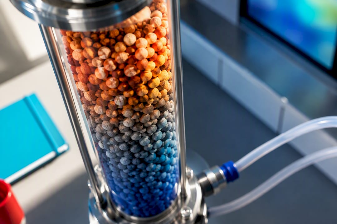
Porous media heat transfer describes how thermal energy moves through a solid matrix and the fluid filling its pores, combining conduction through the skeleton, convection through the fluid, and often radiation across pore surfaces. The single decision that determines everything downstream is whether to treat the solid and fluid as one temperature field (local thermal equilibrium, or LTE) or two coupled fields (local thermal non-equilibrium, or LTNE), and whether to resolve individual pores or average over a representative elementary volume (REV). Get that choice wrong and every Nusselt number, pressure drop, and design decision built on it inherits the error. The sections below walk through how to make that call correctly.
TL;DR:
Using a representative elementary volume is effective only when the sample size is large enough for consistent porosity and properties, especially away from boundaries and thin regions.
The LTE assumption holds when solid and fluid conductivities are similar and interphase heat transfer is rapid; otherwise, LTNE’s two-temperature model becomes necessary.
The effective thermal conductivity in porous media is influenced by advective mixing, stagnant conduction, and microconduction, which vary with porosity, pore size, and material ratios.
Pore-scale simulations are essential for detailed phenomena like contact conduction and temperature hotspots, while REV models suit large-scale, low-gradient flow regimes.
Always perform a pre-simulation LTE/LTNE check, estimate closure parameters, and validate mesh and realization sensitivity to ensure credible porous-media heat transfer results.
Table of Contents
Choosing the Right Physical Scale for Your Model
Every porous-media simulation lives at one of three length scales, and picking the wrong one is the most common reason student projects and even published papers produce results that don’t generalize.
The pore scale resolves individual grains, fibers, or foam struts and the fluid channels between them, typically at the scale of micrometers to a few millimeters. This is where you’d model flow around a single sphere in a packed bed or through one cell of a metal foam. The REV scale (representative elementary volume) averages properties over a chunk of material large enough that porosity, permeability, and effective conductivity become smooth, well-defined numbers rather than wildly fluctuating point values. The region or system scale is the full engineering domain, a packed-bed reactor, a geothermal reservoir, or a heat sink, where you almost never resolve individual pores and instead stitch together REV-averaged behavior.
Finding a valid REV isn’t just a matter of picking a size and moving on. As you grow a sample volume from a single pore, the calculated porosity oscillates wildly at first, then settles into a plateau where adding more material barely changes the number. That plateau is your REV. Below it, your “effective conductivity” or “permeability” is really just a property of one random configuration of grains, not the material.
Practical consequences of getting scale selection wrong show up immediately:
Boundary conditions applied at a pore-scale wall (no-slip, fixed wall temperature) don’t translate directly into REV-scale boundary conditions, which need a Darcy velocity and an effective heat-transfer coefficient instead.
Measured parameters like permeability or effective conductivity only mean something once you know the sample size relative to the pore size. A permeability measured on a 5-grain sample is not the same physical quantity as one measured on a 500-grain sample.
Near solid walls, in thin fins, or in packed beds with a small tube-to-particle diameter ratio, the REV assumption itself can break down because there simply isn’t enough material thickness to average over. Regions like this often need pore-resolved treatment even inside an otherwise REV-scale model, which is one reason coupled multiscale approaches keep gaining ground in the geothermal and metal-foam literature.
For a system with a large domain-to-pore-size ratio, an REV-scale continuum model is almost always the practical choice. For anything with strong local gradients relative to pore size, near a heated wall, around a single foam ligament, inside a thin catalyst pellet, pore-resolved simulation earns its computational cost.
Local Thermal Equilibrium vs. Local Thermal Non-Equilibrium: Picking the Right Formulation
The equilibrium assumption is a modeling convenience, not a law of physics, and it fails more often than most introductory courses suggest.
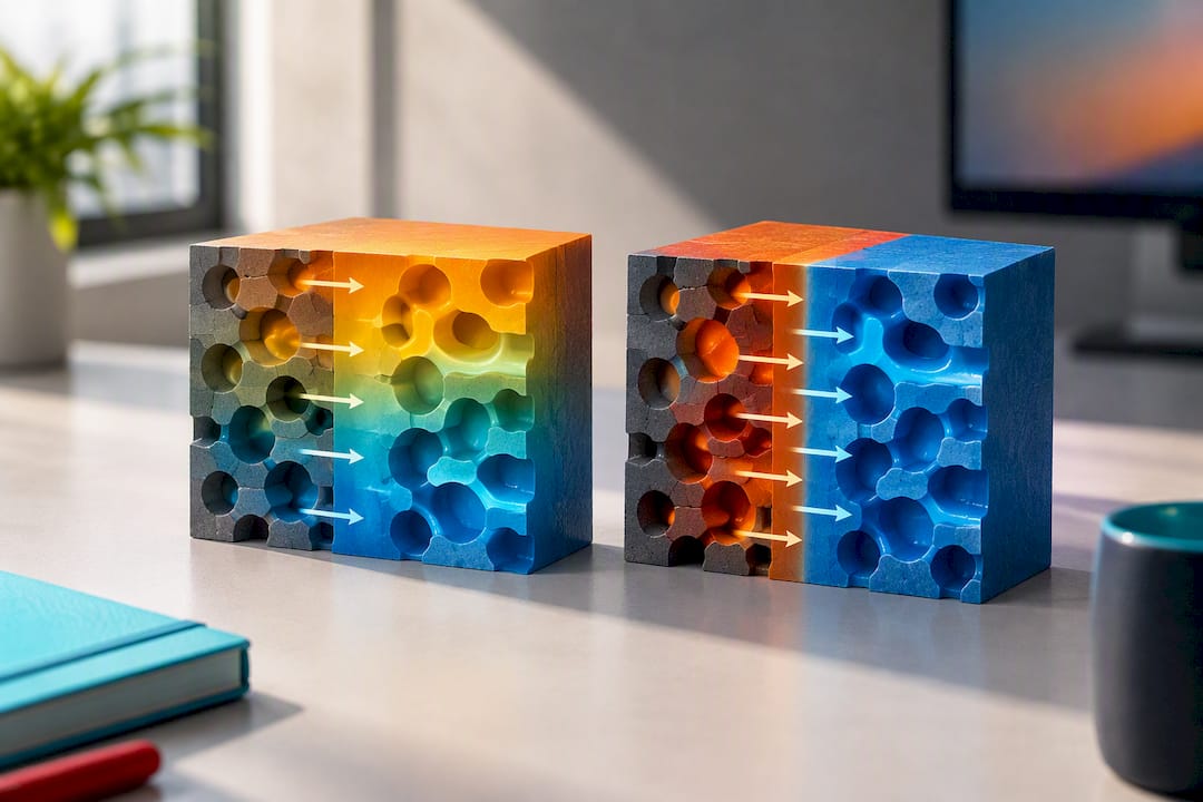
Under LTE, solid and fluid share one temperature field, and you solve a single energy equation weighted by an effective conductivity that blends both phases. Under LTNE, you carry two coupled energy equations, one for the solid phase, one for the fluid, linked by an interphase heat transfer coefficient (often written h_sf) that governs how fast energy moves between them. The two-temperature LTNE formulation is described as follows: the fluid equation balances advection and fluid-phase conduction against the interphase exchange term, while the solid equation balances solid-phase conduction against that same exchange term with opposite sign. When h_sf is very large, the two temperatures converge and LTE becomes an excellent approximation. When it’s small, or when the phases have very different conductivities, the temperatures diverge and LTE quietly produces wrong answers.
A few criteria help you predict which regime you’re in before you run anything:
Conductivity ratio (ks/kf). When solid and fluid conductivities are close, LTE usually holds. Metal foams filled with air (ks/kf in the thousands) are a red flag for LTNE.
Biot-type number for the pore. A modified Biot number comparing interphase heat transfer resistance to intraphase conduction resistance tells you how quickly the phases equilibrate locally.
Flow rate and thermal transient speed. Fast transients, oscillatory heating, or rapid flow through a bed with sluggish interphase exchange all push a system toward LTNE, because there isn’t time for the phases to equalize.
Boundary condition type. Studies applying sinusoidal or heat-flux wall conditions to porous cavities have shown that particle size and porosity strongly change both fluid and solid Nusselt numbers under Darcy-Brinkman-Forchheimer LTNE models, in ways an LTE model simply can’t capture.
Packed-bed reactors running fast exothermic reactions and systems under oscillatory or pulsed heating are the two cases where LTNE most reliably changes the predicted Nusselt number relative to an LTE calculation, sometimes substantially, because the assumption of instantaneous local equilibrium breaks down exactly where the heat transfer coefficient matters most.
Pro Tip: Before committing to a full LTNE simulation, run a quick LTE version first and check the predicted temperature difference between phases at your operating conditions using an estimated h_sf. If that estimated gap stays under a few percent of your total temperature drop across the domain, LTE is probably safe. If it’s larger, don’t trust the single-temperature result.
A short checklist for testing the LTE assumption before you trust a result:
Compute or estimate ks/kf for your material pair.
Estimate h_sf from a correlation or a pore-scale simulation and check the modified Biot number.
Compare characteristic thermal response times of the two phases; if they differ by an order of magnitude or more, treat LTE with suspicion.
If running a transient or oscillatory case, check whether the forcing period is shorter than the interphase equilibration time.
Why Thermal Dispersion Changes What “Conductivity” Even Means
Effective thermal conductivity in a porous medium is never just a volume-weighted average of the solid and fluid conductivities, and treating it that way is one of the most common shortcuts that quietly wrecks accuracy.
Three separate mechanisms combine to produce the effective, or “dispersed,” conductivity you actually measure in a flowing porous system. Advective mixing at the pore scale, fluid parcels taking different tortuous paths at slightly different speeds, spreads heat the way mechanical dispersion spreads a dye front. Stagnant thermal conduction through the solid skeleton and through fluid trapped in dead zones sets a baseline conductivity even at zero flow. Microconduction across contact points between solid grains adds a third, often underestimated, pathway, particularly significant in loosely packed or low-contact-area materials like open-cell foams.
How these mechanisms trade off depends heavily on porosity and geometry:
Higher porosity generally means more fluid-dominated transport and lower solid-solid contact conduction, shifting the effective conductivity toward the fluid’s value.
Larger pore size increases the advective dispersion contribution at a given flow rate, because parcels have more room to take divergent paths.
A high solid-to-fluid conductivity ratio (ks/kf), as in metal foam filled with air, means even modest solid volume fractions dominate the effective conductivity, while a low ratio, like a ceramic packed bed filled with water, shifts the balance toward flow-driven dispersion.
Particle-resolved simulations of packed beds provide one of the clearest quantitative signals in the literature: the global mixing-cup Nusselt number increases with Reynolds number and decreases as porosity increases, a trend that holds across a wide range of bed configurations and gives you a sanity check for any new packed-bed simulation you run. If your model shows Nusselt number rising with porosity at fixed Reynolds number, something in your setup deserves a second look.
A separate, well-documented quirk in packed-bed data is the axial length effect: measured or simulated heat transfer coefficients near the bed inlet differ systematically from values deeper into the bed, because the thermal boundary layer and dispersion pattern haven’t yet reached a periodic, fully developed state. Correlations fit to short experimental beds can overpredict performance if applied naively to longer industrial columns.
When should you measure dispersion directly versus lean on a correlation? If your porosity, particle shape, and Reynolds number fall within the range of a well-validated correlation, like those built into standard packed-bed references, use the correlation and save the compute budget. If you’re working with an unusual geometry (irregular foam, layered beds, non-spherical particles) outside that validated range, a pore-scale simulation or a targeted experiment is worth the extra effort, because extrapolated correlations fail unpredictably outside their fitted domain.
Pore-Resolved Simulation vs. REV-Scale Continuum Models
The choice between resolving every pore and averaging over an REV isn’t just about computational budget. It determines what physics you can even see.
Pore-resolved methods, direct numerical simulation (DNS), particle-resolved CFD, and immersed-boundary approaches, solve the actual Navier-Stokes and energy equations in the real, geometrically complex fluid domain around solid obstacles. They are mandatory when you need local hot spots, contact-point conduction, or detailed interphase heat transfer coefficients that later feed a REV-scale closure. Their cost scales brutally with domain size: resolving a full industrial packed bed pore-by-pore is rarely feasible, so pore-resolved work typically covers a representative sub-domain or a periodic unit cell.
REV-scale continuum models replace the messy pore geometry with averaged fields and a handful of closure relationships. The workhorse equations here are:
Darcy’s law, the simplest closure, valid for low-Reynolds-number, low-porosity flows where viscous drag from the pore walls dominates and inertial effects are negligible.
Brinkman’s extension, which adds a viscous term to Darcy’s law so the model can satisfy a no-slip condition at a solid boundary, essential when you need accurate velocity profiles near a wall rather than just bulk flow rate.
Forchheimer’s inertial correction, which adds a velocity-squared drag term that becomes important at higher Reynolds numbers, where inertial losses in the pore throats start to rival viscous losses.
Dual-porosity models, which split the domain into two interacting continua (a low-permeability matrix and a high-permeability fracture network), standard in fractured-rock geothermal and petroleum applications where a single averaged permeability field can’t capture the real flow pattern.
None of these closures are free. Each one needs parameters, permeability, an interphase heat transfer coefficient, an effective conductivity tensor, and where those parameters come from matters as much as which equation you pick.
Permeability is usually measured experimentally via pressure-drop tests, or estimated from packing correlations (Ergun-type equations for spherical particle beds) when a physical sample isn’t available. The interphase heat transfer coefficient is harder: it’s often backed out from a periodic pore-scale simulation, where you model heat exchange through a single representative unit cell and extract a macroscopic Nusselt number that then defines h_sf for the REV model. A periodic pore-scale transport model built exactly this way shows clearly how solid and fluid material properties propagate up into the macroscopic heat transfer coefficient, which is the cleanest illustration in the literature of how a pore-scale result feeds a REV-scale closure. Effective conductivity closures come either from the dispersion mechanisms discussed above or from a direct pore-scale conduction simulation on a representative sample.
This is the core of a proper multiscale workflow: run a small, well-resolved pore-scale simulation on a periodic or representative unit cell, extract the closure parameters you need, then hand those parameters to a much cheaper REV-scale simulation covering the full engineering domain. Classic reviews of upscaling methods are blunt about the tradeoff involved: REV-scale approaches are semi-empirical, and their accuracy depends entirely on how well the closure relations match the real porous structure you’re actually modeling, not some generic version of it.
Pro Tip: Never reuse a permeability or interphase heat-transfer correlation from a spherical-particle packed bed for a foam or a fractured-rock domain without checking the fit range. Foam ligament geometry and fracture networks produce fundamentally different pore-throat statistics, and a correlation validated on spheres can be off by a wide margin outside that geometry.
Numerical Methods and How to Validate Them Properly
Picking a numerical method for porous-media heat transfer is really about matching the tool to the scale, then proving to yourself, and to anyone reading your results, that the numbers converge and mean something.
At the pore scale, the lattice Boltzmann method (LBM) has become a dominant tool because it handles complex, irregular pore geometries and coupled fluid-thermal transport without the mesh-generation headaches of traditional CFD. At the REV scale, finite element (FEM) and finite volume (FVM) methods remain the standard, particularly for conjugate problems where a porous region couples to a solid wall or an open-flow channel. REV-scale LBM variants have matured too: a cascaded lattice Boltzmann (CLB) formulation gives a more numerically stable alternative to the classic BGK-LBM scheme for convection problems in porous media, particularly useful in higher-Reynolds or anisotropic-permeability cases where BGK can become unstable.
Whichever method you pick, the same set of numerical traps shows up repeatedly in the literature:
Mesh and unit-cell sensitivity. Pore-scale results are notoriously sensitive to mesh resolution around curved solid surfaces and to the size of the representative unit cell chosen; under-resolved random packings produce biased Nusselt predictions, and this sensitivity needs its own dedicated study, not a single mesh check.
Domain periodicity assumptions. Periodic boundary conditions are computationally convenient but only valid if your unit cell genuinely repeats; applying them to a bed with strong wall effects or a low tube-to-particle ratio introduces error that a periodic assumption can’t fix.
Contact and regularization strategies. Spheres or particles that touch at a point create a numerical singularity in most solvers; standard practice is to introduce a small overlap or gap regularization, and the size of that regularization measurably changes local heat transfer near contact points.
Time-step and stability limits. LBM schemes in particular have stability constraints tied to relaxation parameters and local Reynolds number; a time step that’s stable in a low-flow region can go unstable once you push into a higher-Re regime within the same simulation.
Realization averaging. Because packed beds and foams are randomly generated, a single simulation realization can misrepresent the true average behavior; sensitivity studies on randomly packed sphere beds show that Nusselt predictions depend on running multiple packing realizations, not just refining the mesh on one.
For validation, benchmark against published Nusselt correlations for simple geometries (spheres in cross-flow, standard packed-bed correlations) before trusting results on a novel geometry, and cross-check REV-scale closures against a pore-resolved sub-simulation whenever the closure parameters are uncertain. Nield and Bejan’s Convection in Porous Media remains the standard reference point for the correlations and governing-equation forms most validation studies compare against.
Pro Tip: Report your mesh convergence study, your unit-cell size sensitivity, and your number of packing realizations in every write-up, even a student project. Reviewers and future readers (including your own future self debugging the same code) can’t judge whether a Nusselt number of 8.3 means anything without knowing how sensitive it was to those three choices.
A minimal reproducibility checklist before you publish or submit a porous-media heat transfer result: state the mesh resolution and a convergence study, state the number of realizations averaged (for random geometries), state boundary condition type and location, and report a sensitivity check on at least one closure parameter.
Nondimensional Numbers That Define the Flow and Heat Transfer Regime
Five nondimensional groups do almost all the heavy lifting in porous-media heat transfer analysis, and knowing their rough operating ranges saves you from misreading your own results.
The Nusselt number (Nu) compares convective to conductive heat transfer at a surface or pore interface; it’s your primary output metric and the number every correlation ultimately predicts. The Reynolds number (Re), based on either particle diameter or pore-scale velocity, tells you whether flow is viscous-dominated or inertia-dominated. The Rayleigh number (Ra) governs buoyancy-driven natural convection in porous cavities, comparing buoyancy forces to viscous and thermal diffusion. The Darcy number (Da), the ratio of permeability to a characteristic length squared, measures how porous a medium effectively behaves; very low Da pushes a system toward classic Darcy flow, while higher Da signals a need for Brinkman or Forchheimer corrections. The Prandtl number (Pr) sets the ratio of momentum to thermal diffusivity in the fluid phase and rarely changes with the porous structure itself, but it still shapes the thermal boundary layer thickness relative to the velocity boundary layer.
Typical ranges vary enormously by application:
Packed-bed heat exchangers usually operate at particle Reynolds numbers spanning a broad range from low tens up to several thousand, with porosities typical of randomly packed spheres that are often moderate.
Metal-foam heat sinks and pellets studied in the CFD literature commonly run porosities around 0.80 to 0.95, with the particle Reynolds number range of roughly 250 to 2250 covering most practical foam-pellet operating conditions studied to date.
Geothermal reservoirs sit at the opposite extreme: very low Darcy numbers, Rayleigh numbers that determine whether natural convection cells form at all in the rock matrix, and Reynolds numbers so small that Darcy’s law alone is often sufficient.
Moving between pore-scale and REV-scale models means renormalizing your reference length and velocity. At the pore scale, reference length is typically the particle or pore diameter and reference velocity is the actual interstitial fluid velocity. At the REV scale, reference length becomes a domain-scale dimension and reference velocity switches to the superficial (Darcy) velocity, the volumetric flow rate divided by total cross-sectional area, not the pore area. Mixing these two velocity definitions is a common source of Reynolds-number errors that then propagate into wrong Nusselt correlations, so always state explicitly which velocity definition a reported Re or Nu uses.
What the Literature Says About Real Applications
Three application classes dominate the porous-media heat transfer literature, and each one rewards a different modeling priority.
Packed-bed heat exchangers and reactors remain the most studied geometry, partly because spherical particle packings are relatively easy to generate computationally and partly because they’re everywhere in the chemical process industry. The axial length effect discussed earlier means design correlations fit to short laboratory columns need correction before scaling to industrial bed lengths. Pseudohomogeneous models, which lump the bed into an effective medium with a single axial conductivity and an overall radial heat transfer coefficient, remain widely used for transient packed-bed design, but their accuracy depends on selecting effective parameters that actually represent the specific bed geometry rather than generic literature values.
Metal-foam and foam-ring pellets trade some heat transfer performance for dramatically lower pressure drop compared to solid particles, which is exactly why they show up in catalytic reactor retrofits. Particle-resolved CFD studies identifying an optimized foam-ring aspect ratio of 2.5, a cell size near 0.45 mm, and a porosity around 0.82 give a concrete starting point for anyone designing a similar pellet geometry within that same Reynolds number range, rather than starting from an arbitrary guess.
Ground heat exchangers and geothermal reservoirs face a completely different challenge: permeability heterogeneity across the rock matrix, often varying by orders of magnitude between layers, which makes single-permeability REV models unreliable unless the domain is broken into zones or treated with a dual-porosity approach. This is one of the clearest cases where blindly applying a single-scale REV model produces confidently wrong answers.
Design priorities differ by objective:
If maximizing heat transfer is the goal, geometries with relatively higher surface area and carefully balanced porosity generally tend to achieve better heat transfer performance, at the direct cost of pressure drop.
If minimizing pressure drop matters more, foam-based or higher-porosity structured packings usually beat random particle packs at equivalent heat transfer duty.
If the application involves heterogeneous natural media (soil, rock), characterizing spatial permeability variation matters more than refining any single closure parameter.
Your Pre-Simulation Checklist
Before opening any solver, walk through five decisions in order: choose your physical scale (pore, REV, or region), pick governing equations that match that scale (Darcy, Brinkman, Forchheimer, or a two-temperature LTNE set), define boundary conditions consistent with the scale you chose, pull material properties (ks, kf, porosity, permeability) from a reliable source rather than a rough guess, and finish with a mesh or realization sensitivity study plus a validation comparison against a known correlation or published data set.
A convergence run should show your key output, usually Nu or overall pressure drop, changing by a small, stated percentage between your finest two mesh levels, with that percentage reported rather than assumed acceptable. For random packings, three to five independent realizations is a reasonable starting point for checking whether your average Nusselt number has actually stabilized.
Jewlztech built its engineering toolkit around exactly this kind of decision sequence, giving students and early-career engineers a way to run quick conduction, convection, and radiation estimates with a built-in material property database before committing hours of compute time to a full pore-scale or REV-scale simulation. For deeper method background on convection correlations that pair well with porous-media closures, the forced convection in pipes guide covers the correlation math these workflows lean on.
Where the Conventional Advice Gets This Wrong
Most introductory treatments of porous-media heat transfer default to Darcy’s law and LTE because they’re mathematically tractable, then never circle back to check whether that default actually fit the problem. That’s backward. The research consistently shows LTNE and pore-resolved effects matter most exactly in the regimes engineers care about most: fast transients, high conductivity contrast materials like metal foam, and boundary layers near heated walls. Treating LTE as the safe default and LTNE as the exotic exception gets the risk profile inverted.
The field itself has moved past the simple Darcy/LTE starting point, expanding into nanofluids, microfluidic-scale effects, and routine two-temperature formulations as standard practice rather than a specialty topic. If there’s one habit worth building early, it’s running the LTE sanity check outlined above before trusting any single-temperature result, not after a reviewer or a failed prototype forces the question. REV-scale models will always be semi-empirical; the discipline is in knowing which empirical assumption you’re leaning on and whether your geometry actually supports it.
What should come first, before mesh refinement, before choosing a fancier numerical scheme, is scale selection and the LTE/LTNE test. Everything else is downstream of that one choice.
— Joel
Run Your Own Porous-Media Estimates Before Committing to Full Simulation
Every workflow described above needs a fast way to sanity-check parameters before you sink hours into a high-fidelity run, and that’s exactly the gap Jewlztech’s engineering toolkit is built to fill. It combines conduction, convection, and radiation models with a built-in material property database in a single downloadable Excel-based tool, so you can estimate effective conductivity, check a Biot number, or rough out a Nusselt correlation without opening a CFD license or a lattice Boltzmann codebase first.

That matters most for students and early-career researchers who need to test an assumption, like whether LTE holds for their specific ks/kf ratio, before scaling up to a full pore-resolved or REV-scale simulation. The thermal analysis and heat transfer tools cover variable material properties across a wide temperature range, useful for exactly the kind of parameter sweeps this article recommends running before finalizing a model. If your next step is packed-bed or metal-foam design work, the CFD and fluid flow simulation tools extend that same estimate into a fuller flow and heat transfer picture. Start with a quick estimate on the free toolkit, then decide whether your problem actually needs the full simulation.
Sources
For governing equations, scaling arguments, and standard correlations, Nield and Bejan’s Convection in Porous Media is still the reference every serious modeler keeps on the shelf. For pore-scale to REV-scale parameter extraction, the periodic pore-scale transport model paper walks through the actual computation of a macroscopic heat transfer coefficient. For packed-bed benchmark data and length effects, the pore-scale packed-bed simulation study and the metal-foam pellet CFD work both provide concrete geometries and Reynolds ranges worth reproducing as a first validation exercise.
FAQ
What is the difference between LTE and LTNE in porous media?
LTE assumes the solid and fluid phases share one local temperature, solved with a single energy equation and an effective conductivity. LTNE tracks two separate temperature fields linked by an interphase heat transfer coefficient, and it becomes necessary when conductivity ratios are high or thermal transients are fast, as shown in Darcy-Brinkman-Forchheimer LTNE studies.
When should I use pore-scale simulation instead of a REV-scale model?
Use pore-scale simulation when you need local detail, contact-point conduction, or closure parameters like permeability and interphase heat transfer coefficients that a REV model can’t derive on its own. Use REV-scale continuum models (Darcy, Brinkman, Forchheimer) for full-domain engineering problems where computational cost makes pore-resolution impractical.
How does porosity affect heat transfer in packed beds?
Particle-resolved simulations show the global Nusselt number decreases as porosity increases at a fixed Reynolds number, while Nusselt number increases with Reynolds number regardless of porosity. Higher porosity also shifts effective conductivity toward the fluid phase’s value, since there’s less solid-solid contact conduction.
What numerical method is best for porous media heat transfer simulations?
Lattice Boltzmann methods handle complex pore-scale geometries well, while finite element and finite volume methods remain standard for REV-scale and conjugate heat transfer problems. A cascaded lattice Boltzmann formulation offers improved stability over classic BGK-LBM for REV-scale convection cases at higher Reynolds numbers.
Does Jewlztech offer tools for porous media heat transfer calculations?
Jewlztech’s engineering toolkit supports conduction, convection, and radiation analysis with variable material properties and a built-in property database, useful for early-stage parameter estimates. Current pricing for the toolkit is available directly on the Jewlztech site.
Recommended
Comments