
How to Calculate Natural Convection Heat Transfer

Updated: 1 day ago
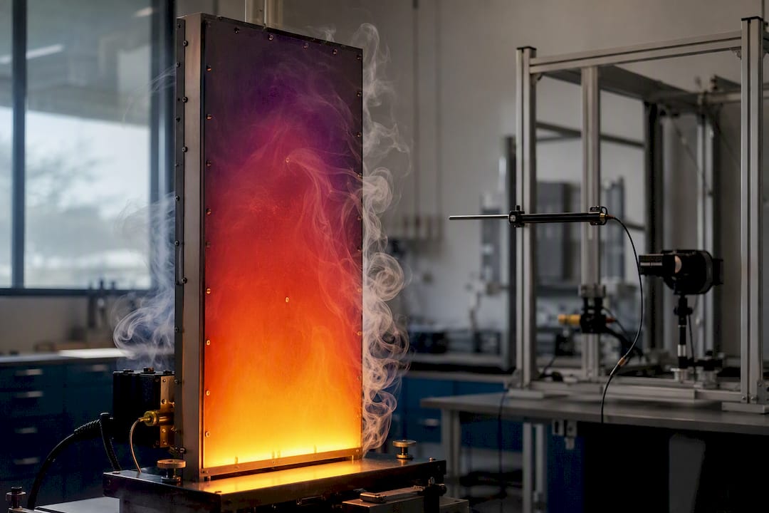
Compute h from the Nusselt number using h = Nu·k/L, then find the heat rate with Q = h·A·ΔT. That’s the entire natural convection calculation in one line. Everything else in this article exists to help you get Nu right, because that single number is where most hand calculations go wrong.
Here’s the fast path from a bare surface temperature to a real answer in watts:
Pick the geometry (vertical plate, horizontal plate, cylinder, sphere) and define the characteristic length L.
Compute the film temperature, Tf = (Tw + T∞)/2.
Pull fluid properties (k, ν, β, Pr) at Tf.
Calculate Grashof (Gr), then Rayleigh, Ra = Gr·Pr.
Match Ra to the right correlation and solve for Nu.
Convert to h, then to Q.
Quick sanity checks before you trust the output: confirm units cancel to a dimensionless Ra, verify Ra sits inside the correlation’s stated range, and check that h for air lands somewhere between roughly 2 and 25 W/m²K. Anything wildly outside that suggests a units slip, not real physics.
Key Takeaways
Getting h right depends on evaluating fluid properties at the film temperature and matching the Nusselt correlation to both the geometry and the Rayleigh number’s valid range.
Point | Details |
Core formula chain | Compute Ra, select the matching Nu correlation, then get h = Nu·k/L and Q = h·A·ΔT. |
Watch the Ra threshold | Vertical plates transition from laminar to turbulent flow around Ra ≈ 1×10⁹. |
Evaluate properties at Tf | Use Tf = (Tw + T∞)/2 for k, ν, β, and Pr to cut property-driven error. |
Check for mixed convection | Calculate Ri = Gr/Re² whenever forced airflow is present nearby. |
Expect 15 to 30% uncertainty | Correlation fit plus property approximation both add error; size designs with margin. |
Automate the chain | The Jewlztech engineering toolkit runs the same Gr to Q calculation with built-in property lookups and unit checks. |
Table of Contents
Natural Convection Calculation: The Core Dimensionless Numbers
Every natural convection calculation runs through three dimensionless groups before you ever touch a Nusselt correlation. Skip this step and you’re guessing at a formula instead of choosing one.
The Grashof number compares buoyancy force to viscous force:
Gr = gβΔTL³/ν²
g is gravitational acceleration (9.81 m/s²), β is the fluid’s thermal expansion coefficient (1/K), ΔT is the temperature difference between surface and fluid (K), L is the characteristic length (m), and ν is kinematic viscosity (m²/s).
The Prandtl number (Pr = ν/α, where α is thermal diffusivity) compares momentum diffusion to thermal diffusion. It’s a pure fluid property, pulled straight from a table at the film temperature, not calculated from your geometry.
Multiply the two and you get the Rayleigh number: Ra = Gr·Pr. This single value tells you whether the flow is laminar or headed toward turbulence, and it’s the input every geometry-specific correlation actually depends on.
The Ra ≈ 1×10⁹ threshold. For a vertical plate, the transition from laminar to turbulent natural convection sits around Ra ≈ 1×10⁹. Below that, boundary layer flow along the plate stays smooth and orderly. Above it, buoyant plumes start breaking into turbulent eddies, and a laminar-only correlation will quietly hand you a wrong answer with no error message attached.
Once you have Ra and a matching correlation, you solve for the Nusselt number, Nu, the ratio of convective to conductive heat transfer across the fluid layer. Convert it to a heat transfer coefficient with h = Nu·k/L, where k is the fluid’s thermal conductivity at Tf. Then Q = h·A·ΔT gives you the actual heat rate in watts, with A as the exposed surface area.
Two things trip people up here. First, L isn’t arbitrary. It’s defined per geometry, and picking the wrong one changes Gr by a cubic factor since L appears as L³, which can shift Ra by an order of magnitude or more. Second, run a quick dimensional check: Gr should reduce to a pure number, Ra should too, and h should come out in W/m²K. If the units don’t cancel cleanly, something upstream is wrong before you even get to the correlation.
Which Nusselt Correlation Should You Use for Your Geometry?
Geometry decides which correlation is valid, and applying a vertical-plate formula to a horizontal cylinder is one of the most common natural convection mistakes engineers make. Each shape has its own characteristic length and its own Ra range where the correlation actually holds.
Vertical flat plate: For laminar flow (10⁴ < Ra < 10⁹), a widely used practitioner shortcut is Nu = 0.59·Ra^0.25, common in electronics cooling work. For a correlation that holds across both laminar and turbulent regimes without a hard switch, the Churchill–Chu equation is the standard choice. L is the plate height.
Horizontal plate, hot side facing up: Uses separate Nu correlations for laminar and turbulent Ra ranges, with L defined as area divided by perimeter.
Horizontal plate, hot side facing down: Convection is suppressed because buoyant fluid can’t easily escape upward, so h runs noticeably lower than the facing-up case at the same ΔT.
Horizontal cylinder: L is the outer diameter, and correlations span a very wide Ra range, from nearly stagnant conditions up through turbulent plumes.
Sphere: Similar treatment to the cylinder, with diameter as the characteristic length and its own King-type correlation.
Inclined plates, enclosed cavities, and finned arrays fall outside these standard forms. For those, either apply an inclination-corrected version of the plate correlation or move to CFD once geometry gets complex enough that a hand correlation stops being trustworthy.
Worked Example: Vertical Plate From Ra to Watts
Take a vertical panel at Tw = 50°C in air at T∞ = 20°C, with height L = 0.2 m and surface area A = 0.5 m².
Film temperature: Tf = (50 + 20)/2 = 35°C ≈ 308 K.
Properties at Tf (air): k ≈ 0.027 W/mK, ν ≈ 1.66×10⁻⁵ m²/s, Pr ≈ 0.71, β ≈ 1/308 K⁻¹.
Grashof number: Gr = gβΔTL³/ν² ≈ 9.81 × (1/308) × 30 × (0.2)³ / (1.66×10⁻⁵)² ≈ 2.75×10⁷.
Rayleigh number: Ra = Gr·Pr ≈ 2.75×10⁷ × 0.71 ≈ 1.95×10⁷.
That Ra sits well inside the laminar range, so Nu = 0.59·Ra^0.25 applies.
Step | Value |
Ra | 1.95 × 10⁷ |
Nu | ≈ 30 |
h | ≈ 5 W/m²K |
Q | ≈ 30 W |
A worked vertical-panel example.html) with comparable inputs produces h ≈ 5 W/m²K and Q ≈ 30 W, matching this result closely and confirming the arithmetic chain holds together.
The most common arithmetic slip here is forgetting to convert Tf to kelvin before computing β, or reusing L instead of L³ inside the Gr formula. Both errors are easy to make and easy to catch: if your h for air lands outside roughly 2 to 25 W/m²K, go back and check those two spots first.
Getting Film Temperature and Fluid Properties Right
Evaluating properties at the film temperature, Tf = (Tw + T∞)/2, is standard practice because property values shift meaningfully across that gap, and using T∞ or Tw alone introduces avoidable error into Nu and h.
For gases, β ≈ 1/Tf (in kelvin) is a good approximation for most engineering work.
For liquids, β comes from a property table, since the ideal-gas approximation doesn’t hold.
Get k, μ, ν, cp, and β at Tf from NIST property tables, a textbook appendix, or a built-in property database in a calculation spreadsheet.
Pro Tip: *If ΔT exceeds roughly 40 to 50°C, or you’re working with a liquid whose properties swing sharply with temperature, run the calculation once at Tf, then check h against a second pass at Tw and T∞ separately.
Unit consistency matters as much as the property values themselves. Keep everything in SI (kelvin for β and Tf, meters for L, watts per meter-kelvin for k) so Gr and Ra come out as clean dimensionless numbers instead of hiding a stray unit conversion three steps downstream.
Should You Use a Calculator or Build the Formula Yourself?
Most online natural convection calculators run the exact same chain you just worked through by hand: film temperature, property lookup, Gr, Ra, Nu, then h and Q. The value they add is speed, not new physics, and reference calculators for standard geometries are a fast way to cross-check a hand calculation.
Before trusting any calculator’s output, confirm three things: it’s using the geometry-correct characteristic length, it’s evaluating properties at Tf rather than at ambient or wall temperature, and its unit system matches yours. A tool that silently assumes English units while you’ve entered SI values will hand you a confidently wrong number.
Run your own worked example through the calculator first and compare Nu, h, and Q against your hand result.
Nudge ΔT or L slightly and confirm the output moves in the expected direction, a basic sensitivity check that catches broken formulas fast.
For repeatable work across many geometries, the Jewlztech Thermalysis Toolkit provides a web-based engineering application that keeps property lookups, correlation selection, and unit handling organized in one integrated environment, rather than requiring engineers to rebuild the calculation chain from scratch each time.
Once geometry gets irregular enough that no standard correlation applies cleanly, that’s your signal to move from a calculator to full CFD.
Common Mistakes That Wreck a Natural Convection Calculation
Most bad results trace back to one of three things: using diameter instead of height as L for a vertical plate, forgetting to convert Tf to kelvin before computing β, or applying a still-air correlation where there’s actually a fan or draft in the room.
Check units first: Gr and Ra must be dimensionless; if they’re not, a unit slipped somewhere upstream.
Sanity-check h against typical air ranges, roughly 2 to 25 W/m²K for natural convection; values far outside that usually mean an error, not exotic physics.
Compute the Richardson number, Ri = Gr/Re², if there’s any forced airflow nearby. Ri near 1 means buoyancy and forced flow are both significant, and a pure natural-convection correlation no longer applies.
Pro Tip: Keep a running note of which correlation you used and its valid Ra range next to every calculation. Six months later, that one line saves you from re-deriving whether your answer was ever trustworthy.
Where Natural Convection Correlations Actually Fall Short
Every Nu correlation in this article carries assumptions that are easy to forget once the numbers start flowing. The laminar/turbulent split at Ra ≈ 1×10⁹ isn’t a hard wall. It’s a transition zone, and correlations near that boundary can disagree with each other by a meaningful margin depending on which dataset they were fit to.
Constant-property assumptions are baked into every standard correlation. Gr, Pr, and Ra are all computed using properties at a single temperature, Tf, even though k, ν, and β all genuinely vary across the boundary layer between the wall and the free stream. For moderate ΔT with air, that approximation holds up fine.
Most correlations also assume laminar or fully turbulent flow with no transitional weirdness, a Newtonian fluid with straightforward property behavior, and a boundary layer that develops without interference from nearby surfaces or airflow. Put a heated plate inside a small enclosure, and reflected buoyant plumes can violate that last assumption entirely, which is part of why enclosure correlations look nothing like open-plate correlations.
None of this makes the correlations unreliable. It means they’re accurate within a defined envelope, and the engineer’s job is knowing where that envelope ends. When your case sits near a Ra transition boundary, has extreme ΔT, or involves obstructed flow, treat the correlation’s output as a first estimate rather than a final number, and validate against a second correlation or a simulation before committing to a design.
When Do You Need Mixed Convection Instead?
Natural convection correlations assume buoyancy is the only thing moving the fluid. The moment there’s a fan, a draft, or any imposed flow nearby, that assumption breaks, and you’re dealing with mixed convection instead.
The Richardson number, Ri = Gr/Re², tells you which regime you’re actually in. When Ri is much greater than 1, buoyancy dominates and a pure natural convection correlation is fine. When Ri is much less than 1, forced convection dominates and you should reach for a forced-convection Nusselt correlation instead. The messy middle ground, Ri near 1, is where neither pure approach works well, and heat transfer can be higher or lower than either mechanism predicts alone depending on whether the forced flow aids or opposes the buoyant plume.

A common real-world trap: electronics enclosures with a small internal fan often sit right in that Ri ≈ 1 zone. Engineers reach for a natural convection formula because the fan feels incidental, then wonder why measured temperatures don’t match the calculation. Even a modest imposed airflow can shift the regime enough to invalidate a pure buoyancy-driven correlation.
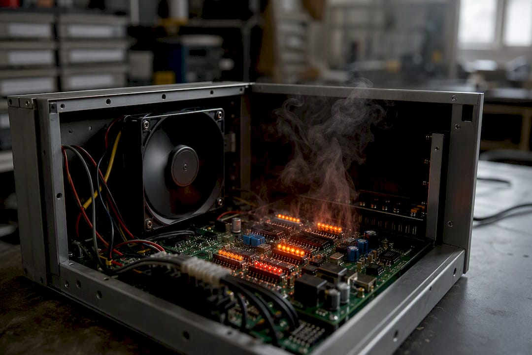
Practical rule: calculate Gr and Re independently before you commit to a correlation family. If Re is nontrivial (there’s measurable forced flow) and Ri lands anywhere near 1, treat the case as mixed convection. Some mixed-convection correlations exist as extensions of the standard Nu = f(Ra) forms, but they require careful sourcing since the assumptions vary by author and by whether the forced and buoyant flows aid or oppose each other. When that data isn’t reliable, a short CFD study settles the question faster than hunting for the right combined correlation.
Does Surface Angle Change the Correlation You Should Use?
Standard correlations cover three orientations: vertical, horizontal facing up, and horizontal facing down. Real hardware rarely sits at exactly one of those angles, and orientation changes h by more than most engineers expect.
Tilt a plate away from vertical and the buoyant boundary layer behavior shifts gradually rather than switching at some sharp angle. Near-vertical inclinations (up to roughly 15 to 20 degrees from vertical) behave close enough to the vertical-plate correlation that using it directly introduces only minor error. Beyond that, the correlation needs an inclination correction, typically applied by adjusting the effective gravitational component acting on the boundary layer, since buoyancy no longer acts purely along the plate’s surface.
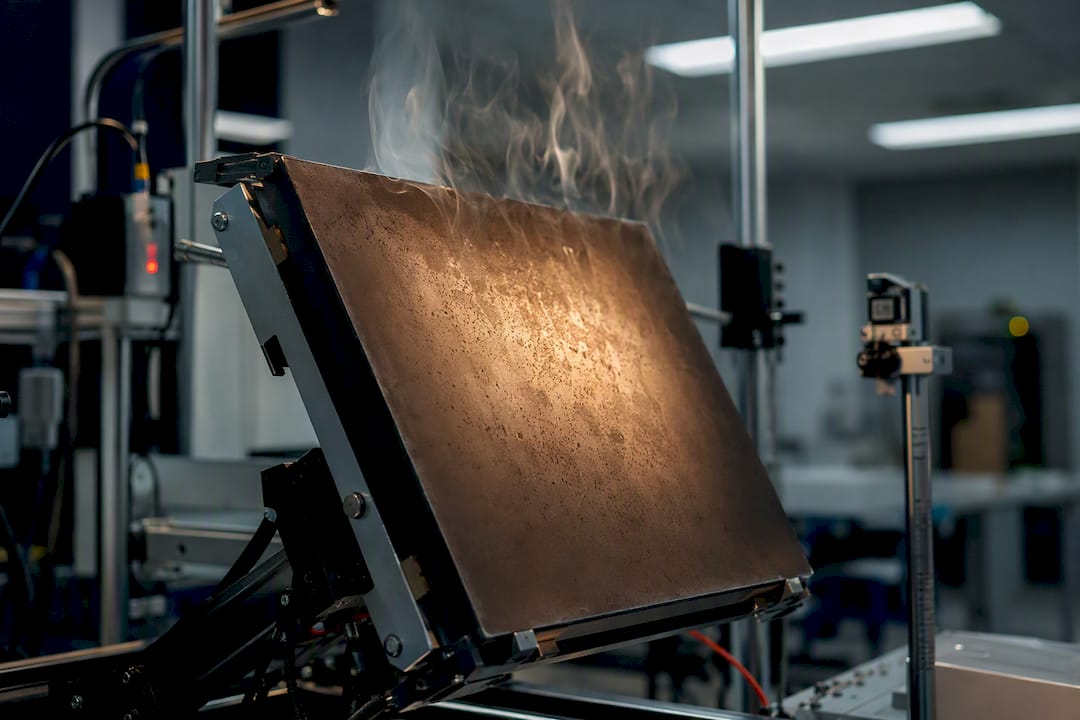
Orientation matters most for horizontal and near-horizontal surfaces. A hot plate facing up lets buoyant fluid rise freely away from the surface, generating strong convective plumes and comparatively high h. Flip that same plate to face down, and buoyant fluid gets trapped against the surface with nowhere to go, forced to escape sideways along the edges instead. The result is a meaningfully lower h at the identical ΔT and area, which is why the two orientations use entirely separate correlations rather than a shared formula with a sign flip.
For anything between roughly 20 and 90 degrees from vertical, engineering practice generally falls back to whichever standard correlation the geometry more closely resembles, then treats the result as an estimate rather than a precise value. If your design tolerance can’t absorb that uncertainty, and many electronics-cooling and enclosure designs can’t, that’s the point where a short CFD run earns its cost.
Constant Heat Flux or Constant Wall Temperature: Which Applies?
Every correlation in this article assumes a constant wall temperature, meaning Tw stays fixed while h and Q respond to it. That’s the right model for a plate held at a set temperature by a controlled heat source, but plenty of real hardware doesn’t work that way.
A resistive heater, a populated circuit board, or a chemical reaction generating heat at a steady rate behaves more like a constant heat flux boundary condition instead, where the heat rate per unit area is fixed and the surface temperature is free to rise or fall in response to how well the fluid carries heat away. Under constant heat flux, correlations exist in a similar Nu = f(Ra) form, but Ra itself gets defined slightly differently since ΔT isn’t known up front. Some formulations use a modified Rayleigh number based on flux rather than temperature difference, and mixing the two conventions is an easy way to get a plausible-looking but wrong answer.
The practical fix for most engineering work: if you know Tw, use the standard constant-wall-temperature correlations covered earlier in this article. If you only know the heat input rate and need to solve for the resulting surface temperature, either find a flux-based correlation designed for exactly that boundary condition, or iterate: assume a Tw, calculate Q, compare it against the known flux, and adjust Tw until they match. That iterative approach is slower than a direct correlation but works with the same Nu formulas you already have, and it’s often the more reliable route when a flux-specific correlation isn’t readily available for your geometry.
Do You Really Need to Go Beyond Film Temperature?
Film temperature is a single-point approximation. It works because it lands roughly in the middle of the property variation between the wall and the free stream, but it’s still a shortcut, not an exact treatment.
For air with moderate ΔT, say under 30 to 40°C, the film-temperature approximation is reliable enough that going further rarely changes the answer meaningfully. Air’s properties don’t swing dramatically over that range, so Tf captures the relevant behavior without extra work.
The picture changes for liquids and for large temperature differences. Viscosity in particular can vary sharply with temperature for many liquids, oils especially, and a single-point property evaluation at Tf can miss that variation entirely. In those cases, engineers sometimes apply a property-ratio correction, adjusting the Nu correlation’s result based on the ratio of a property (commonly viscosity) at the wall versus the free stream, to account for the fact that the boundary layer isn’t behaving like a fluid with uniform properties throughout.
The practical decision point: if you’re working with air and ΔT is modest, Tf alone is fine and further refinement adds complexity without meaningfully better accuracy. If you’re working with a liquid, especially one with strong viscosity-temperature dependence, or ΔT is large enough that the wall and free-stream properties differ substantially, treat the film-temperature result as a starting estimate and either apply a correction factor from the literature or validate against a second method. That second method might be a CFD run with full temperature-dependent properties, which is the only way to fully capture how k, ν, and β actually shift across the entire boundary layer rather than at one representative point.
How Much Error Should You Expect in a Hand Calculation?
Natural convection correlations are empirical fits to experimental data, and every one of them carries some built-in scatter. Understanding roughly how much helps you decide when a hand calculation is good enough and when it isn’t.
Near the middle of a correlation’s range, agreement with experimental data tends to be tighter. Near the laminar to turbulent transition around Ra ≈ 1×10⁹, or near the outer bounds of a correlation’s stated validity, error can run noticeably higher because the underlying physics is genuinely less consistent there.
Property evaluation adds a second layer of uncertainty on top of that. Using film temperature instead of true boundary-layer-averaged properties introduces additional error, generally small for air at moderate ΔT, larger for liquids or large ΔT as covered earlier.
That’s not a reason to distrust hand calculations. It’s a reason to treat their output as a well-founded estimate rather than a precise prediction, and to size designs with enough margin to absorb that range. When a project’s tolerance is tighter than that, cross-check with a second correlation, run a sensitivity study on your key inputs, or move to CFD, where you trade calculation speed for a model that doesn’t carry the same empirical-fit uncertainty baked in from the start.
Why We Default to Film-Temperature Correlations First
Once orientation, enclosures, or mixed flow start introducing uncertainty, that’s the cue to move to simulation. Jewlztech provides web-based engineering applications for thermal analysis and simulation, so engineers can increase model fidelity without rebuilding their workflow from scratch.
— Joel
A Faster Way to Run Repeatable Convection Calculations
Rebuilding the Gr, Ra, Nu, h calculation chain by hand every time you evaluate a new geometry is where small errors can creep in—a mistyped exponent here, a forgotten unit conversion there. The Jewlztech Thermalysis Toolkit provides a web-based engineering application that handles this calculation workflow with integrated material and fluid property data, helping engineers perform repeatable convection calculations without rebuilding the analysis from scratch.

The toolkit includes built-in correlation selection across the standard geometries covered in this article, automatic unit handling so a mismatched input throws a flag instead of a silent wrong answer, and an exportable report you can attach to a design review or hand to a colleague for a second check. It’s the same calculation logic you just walked through by hand, just faster and harder to get wrong. For cases where even that isn’t enough fidelity, orientation extremes, enclosures, mixed convection, the CFD simulation toolkit picks up where hand correlations reach their limit.
Start with the engineering toolkit on your next vertical-plate or cylinder calculation and check the output against the worked example in this article.
Sources
Recommended
Comments