
Engineers: Verify Internal Heat Generation in FEM Without Rebuilding

Updated: 1 day ago
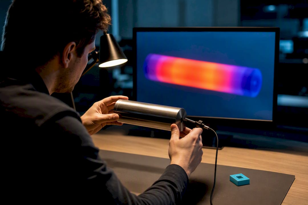
Internal heat generation, denoted q_v and measured in W/m³, is a volumetric source term added directly into the heat conduction equation, not a boundary condition. It raises the local peak temperature (Tmax) above whatever the surface or ambient temperature happens to be, and that rise scales with the square of the conducting path length. Engineers verify any numerical model of it against two closed-form benchmarks: the plane wall and the cylinder solutions, both of which you can compute by hand in under five minutes.
TL;DR:
Internal heat generation is a volumetric source term, measured in W/m³, that raises local temperature above surface or ambient levels depending on the squared length of conduction path.
The key equations for maximum temperature are Tmax = Ts + q_v·L²/(2k) for walls and Tmax = Ts + q_v·r_o²/(4k) for cylinders, with each formula assuming steady-state, uniform generation, and specific boundary conditions.
Q_v often arises from Joule heating, chemical reactions, viscous dissipation, biological metabolism, or radioactive decay, with typical values varying greatly based on the physical process.
Accurate modeling requires applying q_v at the volume level in FEM or CFD tools, confirming units, refining meshes near peaks, and matching boundary conditions to analytical benchmarks.
Verification against closed-form Tmax solutions, like the plane wall and cylinder formulas, is essential for ensuring simulation accuracy before progressing to complex geometries.
Table of Contents
What Internal Heat Generation Actually Means
Internal heat generation is thermal energy produced inside a solid or fluid volume, rather than delivered across its boundary. The standard symbol is q_v (sometimes written as g or S in older texts), and its units are watts per cubic meter (W/m³). That single unit distinction trips up more students than almost anything else in a first heat transfer course, so it’s worth slowing down on.
A surface heat flux, q″, is watts per square meter. It describes energy crossing a boundary, like a wall exposed to solar radiation or a fin losing heat to air. Internal heat generation is fundamentally different: it’s energy appearing inside the material itself, distributed through every cubic meter of volume. Confuse the two, and you’ll apply a q_v value to a surface in your simulation, get a result that’s off by an order of magnitude tied to your part’s thickness, and spend an afternoon debugging a mesh that was never the problem.
There’s a second confusion worth clearing up early: internal heat generation is not the same thing as internal energy. Internal heat generation, by contrast, is a source term in a conduction equation, describing a rate of production, not a stored quantity. One is thermodynamics bookkeeping; the other is a term you add to a PDE.
A few practical notes for keeping q_v consistent across a project:
Always confirm whether a manufacturer or reference value is given per unit volume, per unit mass, or per unit area. A dosimetry or power spec often needs conversion before it’s usable as q_v.
Check dimensional consistency at every substitution. If q_v is in W/m³ and you multiply by a volume in m³, you should recover watts, matching your total power input.
Treat q_v as potentially a function of temperature, q_v(T), whenever the source involves electrical resistance, chemical kinetics, or radioactive decay, since resistivity and reaction rates both shift with temperature.
Treat q_v as a function of time, q_v(t), for transient problems like a battery cell during a fast-charge pulse or a curing resin mid-reaction.
Get the units and the distinction from internal energy locked down early, and everything downstream, the governing equations, the analytical checks, the FEM setup, becomes far less error-prone.
The Governing Equations Behind Internal Energy Production
Every heat conduction problem with an internal source starts from the same general equation, and q_v sits right inside it as an added term:
ρc_p (∂T/∂t) = ∇·(k∇T) + q_v
Here ρ is density (kg/m³), c_p is specific heat (J/kg·K), k is thermal conductivity (W/m·K), and T is temperature. The left side captures how fast thermal energy accumulates in a differential volume; the right side accounts for conduction in and out (the divergence term) plus whatever heat is generated internally. Set constant k and drop the time derivative for a steady-state case, and the equation collapses into the classic Poisson form:
k∇²T + q_v = 0
This is the workhorse equation behind nearly every analytical internal heat generation solution you’ll ever use, including the plane wall and cylinder formulas covered in the next section.
Three things matter when applying this equation to real thermal energy generation problems:
Sign convention. q_v is positive when heat is produced (Joule heating, exothermic reaction) and negative when it’s consumed (an endothermic process, though this is rarer in standard heat transfer coursework). Getting the sign backward silently flips your temperature profile.
Material property placement. ρ, c_p, and k can all vary with temperature in a real material. For a first-pass model, treat them as constants evaluated at a representative operating temperature; for a detailed design check, they need to be functions of T, and your solver needs to iterate to convergence at each time step.
Where q_v applies. It’s defined everywhere inside the domain where generation physically occurs, not at a boundary and not at a single node. This becomes critical once you move into FEM.
In the finite element formulation, q_v enters through the weak form of the governing equation. When you multiply the PDE by a test function and integrate over the domain, the source term becomes a volume integral:
∫_V q_v · N_i dV
where N_i is the shape function for node i. Every element that has q_v assigned to it contributes to the global load vector through this integral, weighted by that element’s own volume. This is the mathematical reason why internal heat generation must be defined as a per-volume quantity in your solver, not a per-node or per-face value. A coarse mesh with large elements and a fine mesh with small elements should both recover the same total generated power for the same q_v, because the volume integral automatically scales the contribution.
For transient runs, the time derivative term means q_v interacts with the thermal mass of the system. A high q_v applied to a low-mass part (thin foil, small electronic die) produces a fast temperature ramp; the same q_v in a large, high-c_p block produces a slow one. This is worth checking with a rough hand calculation, comparing total generated energy against thermal mass, before trusting a transient FEM result blindly.
Verifying Simulations With Analytical Tmax Formulas
The steady-state heat conduction equation with uniform internal heat generation has exact closed-form solutions for two geometries every engineer should have memorized: the infinite plane wall and the infinite cylinder. Both give you a maximum temperature formula you can compute on a calculator, and both are the fastest sanity check available before you trust an FEM result.
Plane wall. For a wall of half-thickness L with uniform q_v and constant conductivity k, symmetric about its centerline, the maximum temperature occurs at the center:
Tmax = Ts + q_v·L²/(2k)
Ts is the surface temperature. The derivation assumes one-dimensional conduction, constant k, uniform q_v throughout the wall, and steady-state conditions with symmetric boundary conditions on both faces. If your real geometry has asymmetric cooling (one face insulated, one face convectively cooled), the peak temperature shifts off-center and this formula only applies as a rough upper bound.
Cylinder. For a solid cylinder of outer radius r_o with uniform q_v, the centerline temperature is:
Tmax = Ts + q_v·r_o²/(4k)
Notice the denominator changes from 2 to 4. That factor-of-two difference comes directly from the geometry: the plane wall solution integrates a one-dimensional Laplacian, while the cylinder solution carries an extra 1/r term from the radial divergence operator. Students who memorize the plane wall formula and just swap in a radius for L get the wrong answer every time, and it’s one of the most common analytical-verification mistakes in a first course.
Both formulas assume a fixed surface temperature Ts as the boundary condition. If your actual problem has a convective boundary instead, you first need to solve for the surface temperature using an energy balance (generated power equals convective heat loss at steady state), then plug that Ts into the Tmax formula. Skipping this step and using ambient temperature directly instead of the true surface temperature is a frequent source of “my simulation doesn’t match the textbook formula” confusion.
Here’s how the two benchmark cases compare:
Parameter | Plane wall | Solid cylinder |
Characteristic length | Half-thickness, L | Outer radius, r_o |
Tmax formula | Ts + q_v·L²/(2k) | Ts + q_v·r_o²/(4k) |
Location of Tmax | Mid-plane (center) | Centerline (axis) |
Denominator constant | 2 | 4 |
Key assumption | 1D conduction, symmetric cooling | Radial conduction, axisymmetric |
Typical use case | Slabs, plates, thick-walled panels | Wires, rods, fuel pins, cylindrical batteries |
A few notes on using these as benchmarks correctly:
Match your simulation’s boundary condition type (isothermal surface vs. convective) exactly to the analytical case, or the comparison is meaningless.
Confirm your FEM model actually has uniform q_v and constant k if you’re comparing against these formulas; a temperature-dependent k requires either a corrected analytical solution or a numerical-only comparison.
Use these formulas for order-of-magnitude sanity checks even on geometries that aren’t perfect walls or cylinders. A rectangular block is often reasonably approximated by an equivalent plane wall for a first-pass Tmax estimate.
Treat any large mismatch between your FEM Tmax and the analytical Tmax, more than a few percent under matched boundary conditions, as a signal to check mesh density, element type, or boundary condition setup before assuming the physics is wrong.
A subtle but common trap is mismatching boundary condition treatment between the analytical case and the simulation. An isothermal wall in the closed-form solution and a convective wall with a very high heat transfer coefficient in the FEM model will look almost identical numerically, but not exactly, and that small systematic offset can look like a modeling bug when it’s really just two slightly different problem statements.
Where Internal Heat Sources Come From in Real Systems
Identifying the physical origin of q_v in your system is what lets you choose a realistic value instead of guessing. The mechanisms fall into a handful of recognizable buckets, and each has a characteristic order of magnitude.
Ohmic (Joule) heating is the most common source engineers model, arising whenever current flows through a resistive medium. Power dissipation follows P = I²R, and dividing by the conducting volume gives q_v. Battery packs are the textbook modern example: cell-level q_v during fast charging or high discharge can reach high values depending on chemistry, current rate, and internal resistance, which is why EV battery thermal management is treated as a dedicated engineering discipline rather than an afterthought.
Chemical and exothermic reaction heat occurs when bond formation in reaction products releases more energy than was required to break the reactant bonds, a fundamental enthalpy relationship that governs everything from curing epoxy to runaway battery decomposition. Reactive systems like curing polymers or packed-bed catalytic reactors can generate q_v values spanning several orders of magnitude depending on reaction rate and concentration, which is exactly why thermal runaway modeling treats q_v as temperature-dependent rather than constant.
Viscous dissipation shows up in high-shear fluid flows, where mechanical energy converts to heat through internal friction. It’s usually negligible in low-viscosity, low-speed flows, but becomes significant in polymer extrusion, lubricant films under heavy load, and high-speed bearing applications, where local q_v can spike sharply in thin shear layers.
Biological and metabolic heat is generated primarily by mitochondria, which account for a large fraction of cellular heat production through oxidative metabolism. The governing source-term concept is identical to the physical cases above, but the property models and spatial distribution differ enough that biomedical thermal modeling is its own specialty rather than a direct copy of electronics cooling work.
Nuclear and radioactive decay heat is the source with the widest dynamic range, from the trace heat of naturally decaying isotopes to the intense, sustained q_v inside a reactor fuel pin, which is precisely the case the cylinder Tmax formula was originally developed to check.
Applying q_v Correctly in FEM and CFD Tools
Getting internal heat generation right in a simulation tool is less about the math, which you now have, and more about avoiding a short list of implementation errors that trip up even experienced users.
Assign q_v at the volume or element level, never as a surface load. Most solvers give you a choice of load type when defining a heat source; internal generation belongs under a volumetric or “body heat generation” category, distinct from a surface flux or convection boundary. Commercial FEM tools implement this as a per-volume input specifically so mesh refinement doesn’t change your total generated power.
Confirm your units before hitting solve. If the software field expects W/m³ and you enter total watts for the part, your result will be wrong by a factor equal to the part’s volume, and it often won’t be obvious from the output alone.
Use a multiplier or lookup curve for temperature-dependent generation. Solvers that support q_v(T) typically let you define a base value plus a scaling curve tied to the local node temperature from the previous iteration, which is standard practice for resistive heating where resistivity rises with temperature.
Refine the mesh where the temperature gradient is steepest, which for internal generation problems is usually near the geometric center or wherever the source density itself is highest. A coarse mesh will systematically under-predict Tmax because it smooths out the peak.
Choose time steps based on the thermal time constant, not on convenience. For fast transient events like a battery pulse, an overly large time step will miss the actual peak temperature entirely, even though the steady-state result eventually converges to the right answer.
The mistakes that show up most often in practice are refreshingly consistent: applying q_v as a surface flux instead of a volumetric load, entering total watts where the software expects W/m³, forgetting that q_v needs updating at every iteration when it’s temperature-dependent, and comparing a convective-boundary simulation against an isothermal-boundary analytical formula without adjusting for the difference.
Pro Tip: Before running a full transient simulation, run a quick steady-state case first and check its Tmax against the plane wall or cylinder formula. If they don’t agree within a few percent, fix that discrepancy before you ever trust the transient results, since the same setup error will just get carried forward through every time step.
Verification and Validation: Proving Your Simulation Is Right
A simulation result without a verification step is a guess with decimal places. The energy-balance check is the fastest one available: at steady state, the volume integral of q_v across the entire domain must equal the net heat leaving through the boundaries. If your solver reports 500 W of total generation but your boundary heat flow only accounts for 470 W, something in your mesh, boundary conditions, or convergence tolerance needs attention.
A workable verification and validation sequence looks like this:
Run the analytical Tmax formula (plane wall or cylinder) for a simplified version of your geometry with matched boundary conditions.
Run the same simplified case in your FEM tool and compare Tmax directly against the analytical value.
Perform a mesh convergence study: rerun the case at two or three progressively finer mesh densities and track how Tmax changes between them.
Compute relative error as (T_FEM − T_analytical) / T_analytical, expressed as a percentage.
Document the mesh density, element type, solver tolerance, and final relative error in your engineering report before applying the same setup to the full, complex geometry.
A thermal safety margin calculation for a pressure vessel deserves a tighter check than an early-stage feasibility estimate.
Mesh convergence itself deserves a specific note: if Tmax keeps shifting by more than a percent or two with each refinement and shows no sign of leveling off, the issue usually isn’t mesh density at all, it’s a boundary condition or material property that’s inconsistent with the physical problem you meant to model.
Worked Examples: Plane Wall, Cylinder, and an FEM Check
Numbers make all of this concrete. Here are two hand calculations followed by the workflow for checking them against a simulation.
Example 1: Plane wall. Consider a plane wall of half-thickness L = 0.02 m (a 4 cm thick slab, symmetric cooling on both faces), thermal conductivity k = 15 W/m·K (typical of a stainless steel alloy), uniform internal heat generation q_v = 2 × 10⁵ W/m³, and a surface temperature Ts = 80°C.
Confirm units: q_v in W/m³, L in meters, k in W/m·K. All consistent.
Apply the formula: Tmax = Ts + q_v·L²/(2k)
Substitute: Tmax = 80 + (2×10⁵ × 0.02²)/(2×15)
Compute the numerator: 2×10⁵ × 0.0004 = 80
Divide: 80 / 30 = 2.67°C
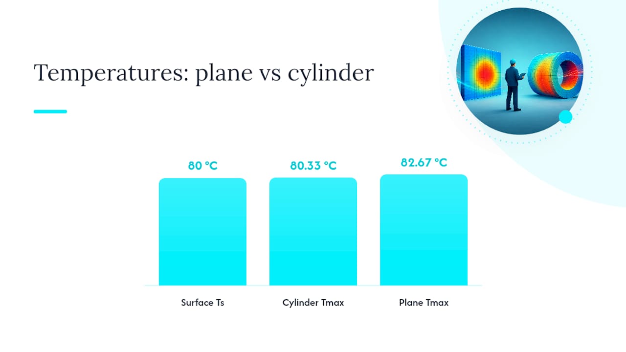
Final result: Tmax = 80 + 2.67 = 82.67°C
Example 2: Cylinder. Now take a solid cylinder of outer radius r_o = 0.01 m (a 2 cm diameter rod), same conductivity k = 15 W/m·K, same q_v = 2 × 10⁵ W/m³, and surface temperature Ts = 80°C.
Apply the formula: Tmax = Ts + q_v·r_o²/(4k)
Substitute: Tmax = 80 + (2×10⁵ × 0.01²)/(4×15)
Compute the numerator: 2×10⁵ × 0.0001 = 20
Divide: 20 / 60 = 0.33°C
Final result: Tmax = 80 + 0.33 = 80.33°C
Notice the cylinder’s Tmax rise is far smaller than the wall’s, even with identical q_v and k. That’s a direct consequence of the characteristic length: the cylinder’s radius is half the wall’s half-thickness in this example, and the temperature rise scales with the square of that length, so a smaller characteristic dimension produces a dramatically smaller peak.
Case | q_v (W/m³) | Characteristic length | k (W/m·K) | Ts (°C) | Tmax (°C) | ΔT rise |
Plane wall | typical q_v value for example | L = 0.02 m | 15 | 80 | Tmax slightly above 80°C | small ΔT rise |
Cylinder | typical q_v value for example | r_o = 0.01 m | 15 | 80 | Tmax slightly above 80°C | smaller ΔT rise |
FEM-check workflow. Set up the same geometry in your solver, matching L or r_o and applying q_v as a volumetric load with the isothermal surface condition at Ts = 80°C. Run the case, extract the peak nodal temperature, and compute relative error against the 82.67°C or 80.33°C benchmark above. If the error exceeds your project’s tolerance, refine the mesh near the center or axis, where the gradient is steepest, and rerun.
Pro Tip: Build your first verification model as a deliberately oversimplified geometry, a true flat plate or a true cylinder, even if your real part isn’t either. Nail the match against the analytical formula first, then add complexity (fillets, holes, asymmetric boundaries) one feature at a time. Debugging one variable at a time is dramatically faster than debugging a fully detailed model that doesn’t match anything.
For readers building out battery or electronics models specifically, the EV battery thermal management guide walks through a similar verification approach applied to a real pack-level geometry, and the heat exchange examples guide covers additional worked problems where volumetric sources interact with convective boundaries.
Behind This Guide: Method and Verification Approach
This guide was built around a straightforward principle: never trust a simulation result you haven’t checked against a closed-form answer. Every formula presented here traces back to the standard steady-state conduction derivation, and every worked example follows the same analytical to FEM to mesh-convergence sequence recommended in the verification section above…
The Thermalysis Toolkit is a web-based engineering application that enables users to evaluate heat-transfer problems using built-in analysis tools and example inputs. Engineers can reproduce known analytical cases such as plane-wall or cylindrical conduction problems before applying the same methods to custom geometries. The toolkit also includes a built-in material property database to simplify conductivity value lookup during calculations.
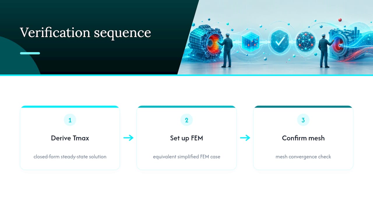
The testing approach behind this article followed the same three-step sequence recommended throughout: derive the analytical Tmax, set up an equivalent simplified FEM case, then confirm mesh convergence before trusting any conclusion drawn from a more complex model.
When to Model q_v Precisely and When to Approximate It
Not every design phase needs a rigorous q_v treatment. A useful gut check: compare the magnitude of internal generation against external heat flux at the boundary. If q_v·V (total generated power) is small relative to the heat already crossing the boundary from convection or radiation, a preliminary sizing model can often treat internal generation as negligible.
The Biot number gives a related intuition. A low Biot number means conduction inside the part is fast relative to convection at its surface, so internal temperature gradients from generation tend to be modest. A high Biot number means the opposite, and that’s exactly when q_v modeling stops being optional.
Battery modules, packed-bed reactors, and dense electronics packages almost always demand precise q_v treatment, because the generation itself is the design driver. A lightly loaded structural bracket with incidental resistive heating usually doesn’t. For early-stage sizing, a rough hand calculation using the plane wall or cylinder formula is often enough to decide which category your project falls into before committing to a full simulation.
— Joel
Verify Your Models Without Rebuilding Them From Scratch
Hand-deriving a plane wall or cylinder Tmax check is fast, but rebuilding that verification workflow from scratch every time you start a new project is where engineers actually lose hours. Jewlztech’s Thermalysis Toolkit provides a web-based engineering application with built-in analytical calculations and a material property database, so the verification process described throughout this guide can be completed efficiently without rebuilding formulas for every project.

The toolkit’s CFD module extends the same approach to cases where viscous dissipation or coupled fluid-thermal effects complicate a pure-conduction model, and the CFD simulation software page walks through what’s included. If your internal generation problem couples to a pressure vessel or cryogenic boundary condition, the cryogenic pressure vessel simulator covers that specific case directly. A monthly subscription provides full access to an engineering toolkit, and free tools and example cases are available to users who wish to try verification cases before purchasing. Visit the engineering toolkit page for more details and current example downloads.
Sources
For the full derivation behind the Tmax formulas used throughout this guide, the BUET lecture notes on internal heat generation walk through both the plane wall and cylinder cases step by step. For the biological side of internal heat production, the Frontiers article on cellular bioenergetics covers mitochondrial heat generation in depth. The ScienceDirect overview of internal energy is worth a read for anyone still untangling internal energy from internal heat generation. For a real-world example of volumetric-equivalent heating in a compact space, Sauna Heater Supply’s sizing guide is a surprisingly good illustration of the same underlying math applied outside a textbook.
FAQ
What is internal heat generation in heat transfer?
Internal heat generation is thermal energy produced within a volume rather than delivered across a boundary, represented by the source term q_v (W/m³) in the heat conduction equation.
What causes internal heat generation inside a material or system?
The main physical mechanisms are ohmic or Joule heating from electrical resistance, exothermic chemical reactions, viscous dissipation in high-shear flows, metabolic heat from biological processes, and radioactive decay in nuclear materials.
How do you calculate the maximum temperature from internal heat generation?
For a plane wall, Tmax = Ts + q_v·L²/(2k); for a solid cylinder, Tmax = Ts + q_v·r_o²/(4k), where Ts is surface temperature, L or r_o is the characteristic length, and k is thermal conductivity.
Can internal heat generation apply to biological systems, not just engineering materials?
Yes. Metabolic heat production in mitochondria follows the same source-term concept, though biological modeling uses different property models and heat distribution patterns than electrical or chemical sources.
Recommended
Comments