
Heat Sink Design: A Practical Engineer's Guide

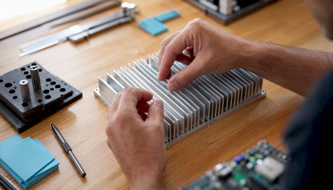
Required sink-to-ambient thermal resistance (θSA) is the single number that determines whether your heat sink design will work. Derive it from the thermal-resistance network before you touch a CAD tool, and you’ll know immediately whether a standard extrusion can solve your problem or whether you need copper, heat pipes, or forced air.
Three quick checks before you go further:
Compute θSA first. Use θSA = (Tj_max − Ta) / Pd − θJC − θCS, where Tj_max is the device’s rated junction temperature, Ta is worst-case ambient, Pd is dissipated power, θJC comes from the datasheet, and θCS depends on your TIM and mounting. The Texas Instruments SLVA462 application note walks through this derivation with worked examples and derating guidance.
Check fin orientation and spacing. Natural convection requires vertical fins spaced sufficiently apart to avoid choking buoyant airflow. Forced convection allows tighter packing but demands pressure-drop budgeting against your fan curve.
Verify your TIM and mounting. Thermal grease typically adds 0.1–0.2°C/W; a dry contact or poorly torqued mount can push θCS above 0.5°C/W and blow your entire thermal budget before the fins do any work.
For complex geometries, multi-source boards, or enclosure interactions, Jewlztech’s Thermalysis Toolkit provides physics-based simulation and parametric sweeps that replace multiple hand-calculation iterations with a single validated model.
Key Takeaways
Effective heat sink design starts with computing the required θSA from the thermal-resistance network and then selecting material, geometry, and manufacturing method to meet that target with adequate margin.
Point | Details |
Compute θSA first | Use θSA = (Tj_max − Ta) / Pd − θJC − θCS before selecting any sink geometry or material. |
Natural convection needs ≥6 mm spacing | Fin spacing below 6 mm chokes buoyant airflow and raises θSA; forced convection allows 2–4 mm with pressure-drop budgeting. |
TIM and mounting are controlled variables | Thermal grease adds 0.1–0.2°C/W; dry contact or poor torque can exceed 0.5°C/W and consume your entire margin. |
Validate with bench test before production | Measure θSA directly at steady state across multiple power steps; a linear ΔT vs. Pd plot confirms the model. |
Thermalysis Toolkit for parametric validation | Jewlztech’s toolkit automates the θSA network, parametric fin sweeps, and test-data overlay to accelerate design iteration. |
Table of Contents
What does heat sink design actually require you to calculate?
How does manufacturing method constrain your heat sink geometry?
How do TIM selection and mounting affect junction temperature?
Natural vs. forced convection: what drives the design choice?
How do you validate a heat sink design through bench testing?
What does heat sink design actually require you to calculate?
Every heat sink design problem reduces to one constraint: keep the device junction temperature below its rated maximum under worst-case operating conditions. The tool for that is the thermal-resistance network, and it runs in series from junction to ambient.
The thermal-resistance network
The series chain is: junction → case → sink → ambient. Each node has a resistance (°C/W) and a temperature drop across it:
ΔT = θ × P
The total network gives:
Tj = Ta + Pd × (θJC + θCS + θSA)
Rearranged for design:
θSA = (Tj_max − Ta) / Pd − θJC − θCS
This is the maximum allowable sink-to-ambient resistance. Any candidate heat sink must meet or beat it. The Texas Instruments SLVA462 note formalizes this network and provides correction factors for orientation and temperature rise that matter when you’re working near the limits.
The three heat transfer modes and when each matters
Conduction moves heat from junction to case and from case through the TIM into the sink base. It’s governed by Fourier’s law: q = k × A × ΔT / L. Sink base thickness and material conductivity directly control this term. A thick copper base spreads heat laterally before it reaches the fins; a thin aluminum base concentrates it.
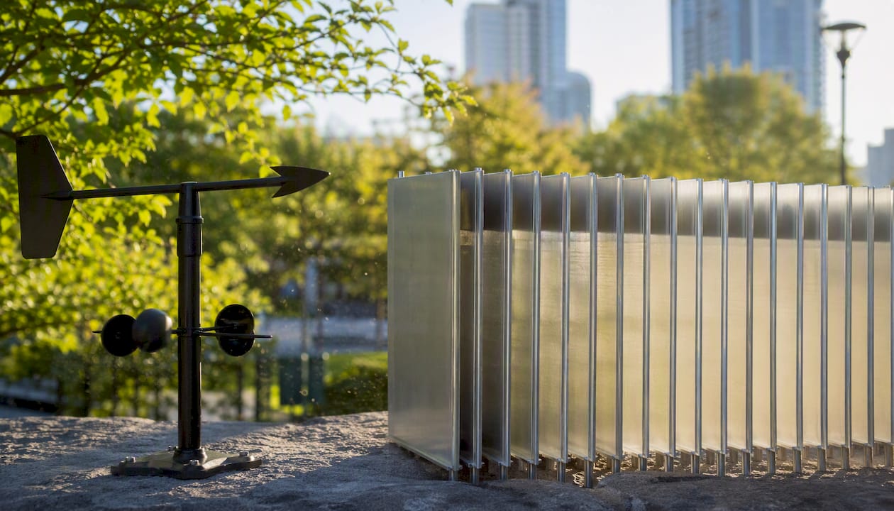
Convection is where the fins do their work. Natural convection relies on buoyancy-driven airflow and is sensitive to fin spacing and orientation. Forced convection uses a fan to drive air through the fin array, which can reduce θSA by several times at moderate airflow compared to natural convection, according to Rftools.
Radiation is often ignored but matters more than engineers expect in passive designs. Texas Instruments’ SLVA462 data shows radiation can account for roughly 25% of total heat dissipation in natural convection at sea level. Black-anodized surfaces improve emissivity and capture that contribution. Under forced airflow, convection dominates and radiation becomes a secondary effect.
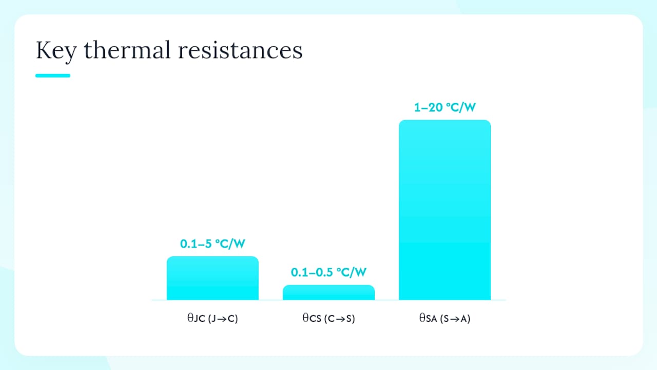
Key thermal parameters at a glance
Parameter | Symbol | Typical Range | Notes |
Junction-to-case resistance | θJC | 0.1–5°C/W | From device datasheet; fixed |
Case-to-sink resistance | θCS | 0.1–0.5°C/W | Depends on TIM and mounting |
Sink-to-ambient resistance | θSA | 1–20°C/W | Your design target |
Max junction temperature | Tj_max | 125°C | From device datasheet |
Worst-case ambient | Ta | 40°C | Application-specific |
Steady-state vs. transient: The network above is steady-state. For pulsed loads, you need thermal impedance (ZθJC) curves from the datasheet and a transient analysis. Most power electronics designs target steady-state first, then verify transient margins separately.
For a deeper look at the underlying physics and math, Jewlztech’s guide to heat transfer models covers conduction, convection, and radiation correlations in detail.
Which material should you choose for your heat sink?
Choose the material that matches your thermal conductivity requirement, mass budget, manufacturing process, and unit cost. Aluminum handles the vast majority of applications. Copper earns its cost premium only when you need roughly twice the conductivity in the same volume, or when spreading resistance from a small, high-flux source is the binding constraint.
Material properties compared
Mersen’s high-power design guide confirms that copper offers approximately twice the thermal conductivity of aluminum, which translates directly to lower spreading resistance when the heat source footprint is small relative to the sink base.
When copper is worth it
Copper makes sense when a high-flux source (say, a 10 mm × 10 mm die dissipating 100 W) sits on a large base and spreading resistance in aluminum would raise junction temperature by several degrees. It also suits applications where sink volume is tightly constrained and you need every watt of conductivity. The weight penalty (roughly 3.3× denser than aluminum) and cost premium are real trade-offs. In most board-level designs, aluminum wins on cost and manufacturability.
Heat pipes and vapor chambers
Heat pipes and vapor chambers don’t replace fins. They move heat from a concentrated source to a larger fin array that can reject it more effectively. A heat pipe embedded in an aluminum base can spread heat across a fin array two or three times the source footprint, effectively reducing spreading resistance to near zero. Vapor chambers do the same in two dimensions and suit large, flat heat sources.
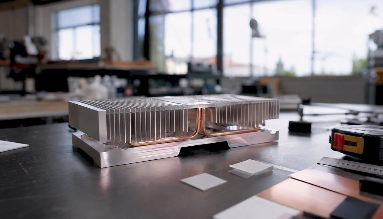
Choose heat pipes or vapor chambers when the source footprint is small, the available sink footprint is large, and spreading resistance in a solid base would consume too much of your θSA budget. For a structured comparison of when to escalate to these solutions, see Jewlztech’s guide on alternative cooling solutions.
Emerging materials
Graphene-enhanced composites and carbon-fiber-reinforced aluminum show thermal conductivity values well above copper in the in-plane direction, but anisotropy, cost, and joining complexity limit them to aerospace and high-reliability electronics today. Metal-matrix composites (aluminum/SiC) offer a better CTE match to silicon than pure aluminum, which reduces thermal-cycling stress at the die attach. Both are proven in niche applications but not yet cost-competitive for general power electronics.
Pro Tip: When running a parametric design sweep, include material conductivity as a variable alongside fin spacing and ambient temperature. A simulation that compares aluminum vs. copper at three fin spacings in one run often reveals that a slightly larger aluminum sink outperforms a smaller copper one at a fraction of the cost.
How do fin geometry choices affect thermal performance?
Fin spacing and orientation drive convection performance more than fin count does. Packing more fins into the same envelope without accounting for airflow restriction is one of the most common ways a heat sink design fails to meet its θSA target in test.
Plate fins vs. pin fins
Plate (straight) fins are the default for most extrusion-based designs. They’re easy to manufacture, have predictable pressure-drop behavior, and work well when airflow is unidirectional. They’re the right choice for most forced-convection applications with a defined airflow direction.
Pin fins excel when airflow direction is uncertain or multidirectional, as in natural convection with variable orientation or in open enclosures. Pins create turbulence that improves convective heat transfer coefficients, but at the cost of higher pressure drop for a given fin density. They’re harder to extrude and typically require casting, machining, or additive manufacturing. For a detailed technical treatment of pin-fin geometry, Jewlztech’s pin fin guide covers aspect ratios, spacing rules, and application trade-offs.
Design rules for fin geometry
Natural convection fin spacing: ≥6 mm (0.25 in). Below this threshold, buoyant airflow is choked and θSA rises sharply. Mersen’s design guide and the MDPI Energies geometry optimization study both confirm this as the practical lower bound.
Forced convection fin spacing: 2–4 mm is typical. Tighter spacing increases surface area but raises pressure drop, which requires a higher-static-pressure fan.
Fin height-to-spacing ratio: Keep below 10:1 for natural convection to avoid flow stagnation at fin tips. Forced convection tolerates higher ratios.
Fin thickness: 1–2 mm for extruded aluminum is standard. Thinner fins are achievable with skiving or bonded construction and increase surface area, but add manufacturing cost.
Fin tip clearance: Maintain at least 5 mm between fin tips and any enclosure wall to avoid recirculation that raises effective ambient temperature.
Volumetric resistance and packing density
Adding fins increases surface area, but it also increases flow resistance. At some packing density, the reduction in airflow through the fin channel outweighs the gain in surface area, and θSA stops improving. This optimum depends on fan curve, fin height, and channel length. Hand calculations can estimate it; CFD confirms it.
Quick geometry assessment checklist
Before committing to a fin geometry for simulation or prototyping, check these:
Fin orientation aligned with gravity (natural convection) or with primary airflow direction (forced convection)?
Fin spacing ≥6 mm for natural convection, or pressure-drop budget confirmed for forced convection?
Height-to-spacing ratio below 10:1 for natural convection?
Fin tip clearance ≥5 mm from enclosure walls?
Base thickness sufficient to spread heat to the full fin array without excessive conduction ΔT?
Geometry Parameter | Natural Convection | Forced Convection |
Min fin spacing | ≥6 mm | 2–4 mm |
Fin height-to-spacing ratio | ≤10:1 | Up to 20:1 |
Preferred fin type | Plate (vertical) | Plate or pin |
Fin thickness (extruded Al) | 1.5–2 mm | 1–2 mm |
Base thickness | 3–6 mm | 3–5 mm |
How does manufacturing method constrain your heat sink geometry?
The manufacturing process sets the achievable fin density, tolerances, and cost at your production volume. Designing a fin geometry that only a machining center can produce, then discovering your volume requires extrusion, is an expensive mistake.
Manufacturing methods and their trade-offs
Extrusion is the workhorse. It produces consistent, repeatable profiles at low per-unit cost for medium-to-high volumes. Minimum fin thickness is typically 1.2–1.5 mm for aluminum, minimum spacing around 2–3 mm, and maximum aspect ratio (fin height / fin thickness) around 6:1 to 8:1. Complex cross-sections are possible but increase die cost.
Skiving cuts fins from a solid base using a blade, producing very thin fins (down to 0.3 mm) at high aspect ratios (up to 20:1 or more). It’s the method of choice when you need high fin density in aluminum or copper without bonding. Lead times are moderate and setup costs are lower than extrusion tooling for small runs.
Bonded and soldered fins attach separately formed fins to a base, enabling taller fins and finer spacing than extrusion allows. Mersen’s design guide identifies bonded and soldered construction as the route to high-performance fin arrays for high-power applications. The thermal resistance of the bond joint is an additional term in the conduction path and must be accounted for in the θSA calculation.
Stamped and formed fins suit high-volume, low-cost applications where fin geometry is simple. Tolerances are looser than machined or skived fins, and the process is limited to thinner materials.
Machined (milled) fins offer the tightest tolerances and the most geometric freedom, but at the highest per-unit cost. Use for prototypes, low-volume custom designs, or when no other process can achieve the required geometry.
Geometric limits by manufacturing method
Secondary operations
Anodizing protects aluminum from corrosion and improves surface hardness. Black anodizing raises surface emissivity to approximately 0.85–0.9, which meaningfully increases radiative heat transfer at large temperature differentials. Under high forced airflow, the radiative gain is marginal and may not justify the added process step.
Mechanical finishing (lapping or milling the base) reduces surface roughness and improves contact conduction at the TIM interface. When base flatness exceeds 50 µm across the contact area, lapping is worth the cost.
Early DFM checklist
Confirm the required fin spacing and thickness are achievable with your target process.
Get vendor datasheets with actual geometric tolerances, not nominal values.
Check whether your fin height-to-thickness ratio falls within the process’s aspect-ratio limit.
Identify whether secondary operations (anodize, lap, plate) are needed and add them to the cost model.
For bonded or soldered fins, request bond-joint thermal resistance data from the vendor.
Step-by-step heat sink sizing: a worked example
Result first: for a 50 W device with Tj_max = 125°C, Ta = 50°C, θJC = 0.5°C/W, and θCS = 0.2°C/W (thermal grease, properly torqued), the required θSA is 0.8°C/W. That rules out natural convection for any reasonably sized sink and points directly to forced air with a moderate fin density.
Here’s how to arrive at that number and what to do with it.
Core formula set
Allowable junction temperature rise: ΔT_total = Tj_max − Ta
Required θSA: θSA = ΔT_total / Pd − θJC − θCS
Junction temperature check: Tj = Ta + Pd × (θJC + θCS + θSA_actual)
Safety margin: ΔT_margin = Tj_max − Tj_calculated (target ≥10°C)
Worked example: step by step
Step 1 — Define the inputs.
Pd = 50 W (device power dissipation)
Tj_max = 125°C (from device datasheet)
Ta = 50°C (worst-case ambient, including enclosure temperature rise)
θJC = 0.5°C/W (from device datasheet)
θCS = 0.2°C/W (thermal grease, per onsemi AND9859 guidance)
Step 2 — Compute allowable ΔT. ΔT_total = 125 − 50 = 75°C
Step 3 — Compute required θSA. θSA = 75 / 50 − 0.5 − 0.2 = 1.5 − 0.7 = 0.8°C/W
Step 4 — Check against natural convection range. Natural convection extruded sinks typically fall in the 3–20°C/W range. At 0.8°C/W, natural convection is not viable for a compact sink. Forced air is required.
Step 5 — Select a candidate sink. From manufacturer curves, a forced-air sink with a 120 mm × 80 mm × 40 mm fin array at 400 LFM airflow achieves approximately 0.7°C/W. That provides a 12.5°C safety margin at the junction (Tj = 50 + 50 × (0.5 + 0.2 + 0.7) = 50 + 70 = 120°C).
Step 6 — Apply ambient derating. If the enclosure raises local ambient by 5°C above room temperature, Ta becomes 55°C. Recalculate: Tj = 55 + 70 = 125°C. Margin is now zero. Either improve enclosure venting, reduce θCS, or select a lower-θSA sink.
Step 7 — Verify with manufacturer curves. Published θSA values in datasheets are typically measured at a specific orientation and airflow. Apply correction factors from the Infineon AN-1057 application note for length, temperature rise, and orientation before finalizing your selection.
Calculation checklist
Check | Action |
Worst-case Ta confirmed? | Include enclosure rise, not just room ambient |
θJC from current datasheet? | Verify against latest revision |
θCS matches TIM and mounting? | Use measured or vendor-specified value |
Safety margin ≥10°C? | If not, revisit TIM, airflow, or sink size |
Manufacturer curve at actual airflow? | Apply correction factors for orientation |
For additional worked examples across different device types and power levels, Jewlztech’s heat exchange examples guide provides practical case studies.
How do TIM selection and mounting affect junction temperature?
Mounting and TIM selection can shift junction temperature by 5–10°C in a 50 W design. θCS is not a fixed constant you read once and forget. It’s a controlled design variable that depends on TIM type, surface finish, mounting pressure, and whether the assembly is consistent across production units.
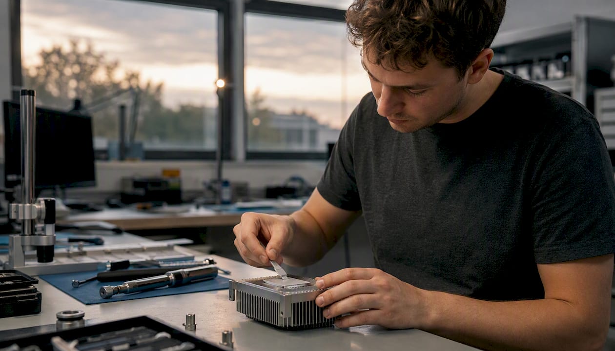
TIM types and typical θCS values
Per onsemi’s AND9859 mounting guide, thermal grease reduces both contact resistance and its sensitivity to mounting torque variation, which matters for production consistency.
Mounting torque and pressure
For TO-220 packages, the recommended torque range is approximately 4–6 kgf·cm. Below that range, contact pressure is insufficient and θCS rises. Above it, package deformation can worsen contact and risk mechanical damage. Larger packages (such as TO-247 or D²PAK) typically accept higher torque, around 9 kgf·cm, but always verify against the specific package datasheet.
Washer and clamp hardware affects pressure distribution. A spring washer maintains consistent pressure over thermal cycles; a flat washer does not compensate for creep in the TIM layer. For high-reliability designs, spring-loaded clamps are preferable to screw-only mounting.
Surface finish and flatness
A machined or lapped base surface with flatness better than 25 µm across the contact area minimizes the void fraction in the TIM layer and keeps θCS near its rated value. Anodized surfaces add a thin dielectric layer that slightly increases contact resistance compared to bare aluminum. When electrical isolation is not required, bare aluminum with thermal grease is the lowest-resistance option.
Pro Tip: Measure θCS directly during prototype validation by placing a thermocouple at the case and one at the sink base, then computing (Tcase − Tsink) / Pd. If the measured value exceeds your design assumption by more than 0.1°C/W, investigate surface flatness, TIM coverage, and torque before attributing the discrepancy to the sink itself.
Mounting checklist
TIM type selected and θCS value confirmed from vendor datasheet?
Mounting torque specified on assembly drawing and verified with a torque wrench?
Surface flatness of sink base measured or specified to vendor?
Rework procedure defined (especially for grease: clean and reapply)?
Production consistency plan in place (torque control, TIM dispense volume)?
Natural vs. forced convection: what drives the design choice?
Natural convection requires vertical fins with at least 6 mm spacing. Forced convection allows tighter fins but needs pressure-drop budgeting against the fan curve. The choice between them is usually settled by the required θSA: if your target is below roughly 3°C/W, natural convection is off the table for any practical sink size.
Reading a fan curve and matching it to your fin array
A fan’s performance curve plots static pressure (in inches H₂O or Pa) against volumetric flow rate (CFM or m³/hr). Your fin array has a system resistance curve that rises with flow rate. The operating point is where the two curves intersect.
To estimate fin array pressure drop for a quick check, use the channel flow approximation:
ΔP ≈ f × (L / Dh) × (ρ × V²) / 2
where f is the friction factor (approximately 96/Re for laminar flow in rectangular channels), L is fin length, Dh is hydraulic diameter of the fin channel, ρ is air density, and V is mean channel velocity. For most board-level forced-convection designs, a fan delivering 100–300 LFM through a 40–80 mm fin array is the starting point.
Converting between LFM and CFM: CFM = LFM × (fin array cross-section area in ft²). A 100 mm × 50 mm fin array face has an area of approximately 0.054 ft², so 200 LFM through it equals roughly 10.8 CFM.
Pressure-drop trade-offs
Tighter fin spacing increases surface area and improves heat transfer, but raises pressure drop. A fan operating against higher static pressure delivers less flow, which partially offsets the surface-area gain. The net effect on θSA depends on where you are on the fan curve.
Orientation and enclosure layout
For natural convection, fins must be vertical and aligned with the buoyancy-driven airflow direction. Horizontal fins trap hot air between them and can double θSA compared to vertical fins of the same geometry. The Infineon AN-1057 note provides orientation correction factors that quantify this effect.
Place heat-generating devices toward the top of enclosures for natural convection, and keep inlet vents at the bottom and outlet vents at the top. Blocking the outlet vent is the single most common enclosure layout mistake: it raises effective ambient temperature by recirculating hot air.
For forced convection, align the fin channels with the fan’s airflow direction and leave at least one fin-height of clearance at the inlet and outlet to avoid flow separation. For a structured comparison of when to choose fans vs. passive cooling, Jewlztech’s active vs. passive cooling guide covers the decision criteria in detail.
Key figure: Radiation accounts for roughly 25% of heat dissipation in natural convection at sea level, per Texas Instruments’ SLVA462 data. At altitude, lower air density reduces convective performance and increases the relative contribution of radiation, which means black-anodized surfaces matter more in high-altitude deployments.
Natural vs. forced convection quick-reference
Natural convection: fin spacing ≥6 mm, vertical orientation, θSA typically 3–20°C/W.
Forced convection: fin spacing 2–4 mm, aligned with airflow, θSA improvement of roughly 3–5× at moderate airflow.
Hybrid (fan-assisted natural convection): useful when noise constraints limit fan speed; operates near the natural-convection regime but with a low-speed fan to improve flow.
Liquid cooling: for θSA targets below 0.5°C/W where air cooling cannot deliver.
How do you validate a heat sink design through bench testing?
Validate θSA and junction temperature with controlled power input, stable ambient, and repeatable sensor placement. A test that skips any of those three conditions produces numbers you cannot trust or reproduce.
Test protocol: step by step
Thermal soak. Allow the assembly to reach ambient temperature before applying power. Minimum soak time is typically 30 minutes in a controlled environment.
Controlled power input. Use a precision DC power supply and measure actual dissipated power (V × I), not programmed setpoint. Account for lead resistance if relevant.
Steady-state confirmation. Apply power and monitor temperatures until the rate of change is less than 0.5°C over 5 minutes. Record temperatures only at steady state.
Power steps. Run at 25%, 50%, 75%, and 100% of rated power. Plot ΔT vs. Pd; the slope is θSA. A linear relationship confirms the model; nonlinearity suggests a contact or flow problem.
Sensor placement. Place the case thermocouple at the center of the device footprint, as close to the package as possible without blocking the TIM. Place the ambient sensor at least 150 mm from the sink in undisturbed air.
Repeatability check. Run the same power step three times. If θSA varies by more than 5% between runs, investigate sensor placement, TIM consistency, or ambient stability.
Sensor placement and junction temperature inference
Direct junction temperature measurement is rarely possible in production packages. Infer Tj from the datasheet’s θJC and the measured case temperature:
Tj_inferred = Tcase + Pd × θJC
For power MOSFETs and IGBTs, the on-state voltage (Vds or Vce) at a known current is a calibrated temperature indicator and can serve as a non-invasive Tj measurement if you calibrate it at a known temperature first.
Data recording template
Environmental control notes
Altitude reduces air density and convective capacity; a design validated at sea level needs derating at 2,000 m or above. Always record ambient conditions (temperature, humidity, altitude) alongside thermal data so results are reproducible and comparable.
When should you use hand calculations vs. CFD simulation?
Use hand calculations for feasibility checks. Move to CFD when geometry, multiple heat sources, or enclosure recirculation break the linear assumptions that make hand calculations valid.
The decision isn’t about precision preference. It’s about whether the physics of your problem fit the model. A single device on a flat sink in open air fits a hand calculation well. A multi-chip module in a sealed enclosure with recirculating flow does not.
The escalation path
Hand calculation (θ network, ΔT = θ × P): use for initial sizing, quick trade-off comparisons, and sanity checks on vendor-supplied θSA values. Takes minutes.
Lumped-network model (multi-node RC network): use when you have several devices on one sink, or when you need to model transient response. Tools like spreadsheet-based solvers or simple simulation scripts handle this tier. Jewlztech’s Thermalysis Toolkit operates at this level and above, with a built-in material database and automated θSA calculators that replace manual network assembly.
2D/3D CFD: use when fin interaction, enclosure recirculation, or non-uniform heat sources produce flow patterns that lumped models cannot capture. CFD is also the right tool when you’re optimizing fin geometry for minimum pressure drop at a fixed θSA target, as the MDPI Energies geometry optimization study demonstrates for topology-based approaches.
Validation workflow
A simulation that hasn’t been benchmarked against test data is a model, not a validated design tool. Follow this sequence:
Run the hand calculation and confirm the result is physically plausible.
Build the CFD model with the same boundary conditions (power, ambient, airflow).
Check mesh convergence: refine the mesh until θSA changes by less than 2% between refinement levels.
Compare CFD output to bench test data. If they agree within 10%, the model is validated for that geometry class.
Sensitivity analysis: vary boundary conditions (±10°C ambient, ±20% airflow) to confirm the design has adequate margin across its operating range.
Pro Tip: The most common CFD error in heat sink modeling is applying a uniform heat flux across the entire device footprint when the actual die is much smaller than the package. Use the die footprint, not the package footprint, as the heat source in your model. The difference in spreading resistance can be 0.2–0.5°C/W.
Common simulation pitfalls
Applying adiabatic boundary conditions to enclosure walls when the walls actually conduct heat.
Using still-air ambient conditions for a forced-convection model.
Ignoring radiation in natural-convection models (it contributes roughly 25% of dissipation).
Treating θJC as a lumped resistance when the die is offset from the package center.
Skipping mesh convergence and accepting the first result.
For context on simulation tool choices, Jewlztech’s comparison of SimScale alternatives covers where physics-based tools fit into a practical engineering workflow.
What are the most common heat sink design mistakes?
Follow an iterative workflow that locks the thermal budget early and validates at each milestone. The designs that fail in test almost always skipped one of the early checks, not the final CFD run.
The design workflow
Define requirements: Pd, Tj_max, Ta_worst, available envelope, airflow constraints, and lifetime/reliability targets.
Hand-calc feasibility: compute θSA, check against natural vs. forced convection ranges, confirm material and manufacturing are viable.
Manufacturability check: verify fin geometry is achievable with the target process and get vendor confirmation on tolerances.
Prototype and test: build to the hand-calc geometry, measure θSA and Tj, compare to predictions.
Simulation validation: if test and hand calc agree, the model is validated. If not, investigate before proceeding.
Production verification: confirm that production assembly (TIM dispense, torque, surface finish) matches prototype conditions.
Common pitfalls and how to fix them
Ignoring θCS. Engineers often treat θCS as zero or use a generic 0.2°C/W without verifying it for their specific TIM and mounting. Measure it directly during prototype validation.
Assuming datasheet θSA orientation. Published θSA values are measured at a specific orientation (usually vertical fins, free air). Using that number for a horizontal or enclosed installation without correction overstates performance.
Poor vent layout. Blocking the outlet vent or placing inlet and outlet vents on the same side of an enclosure creates recirculation that raises effective ambient temperature by 5–15°C.
Overpacking fins in natural convection. Spacing below 6 mm chokes buoyant airflow and raises θSA. More fins in the same envelope can make performance worse, not better.
Underestimating worst-case Ta. Room temperature is not worst-case ambient. Add enclosure temperature rise (typically 5–15°C above room), solar loading for outdoor equipment, and end-of-life fan degradation for forced-convection designs.
Neglecting thermal cycling stress. Repeated power cycling creates mechanical stress at the TIM interface and die attach due to CTE mismatch. For designs with >10,000 power cycles over their lifetime, specify a TIM with low modulus and verify bond-line thickness.
Quick reference: formulas, material properties, and lookup tables
The formulas below are the ones you’ll reach for repeatedly. Units are stated with each.
Core equations:
θSA = (Tj_max − Ta) / Pd − θJC − θCS [°C/W]
ΔT = θ × P [°C = (°C/W) × W]
Tj = Ta + Pd × (θJC + θCS + θSA) [°C]
Fourier’s law (conduction): q = k × A × ΔT / L [W = (W/m·K) × m² × °C / m]
Newton’s law (convection): q = h × A × (Ts − Ta) [W = (W/m²·K) × m² × °C]
Stefan-Boltzmann (radiation): q = ε × σ × A × (Ts⁴ − Ta⁴) [W; σ = 5.67 × 10⁻⁸ W/m²·K⁴]
Material properties quick reference:
Fin spacing quick rules:
Natural convection: ≥6 mm (0.25 in) minimum
Forced convection (low static pressure fan): 3–4 mm
Forced convection (high static pressure fan): 2–3 mm
Typical θSA ranges:
Natural convection, extruded aluminum: 3–20°C/W depending on size
Forced air at moderate flow: roughly 3–5× improvement over natural convection baseline
Mounting torque quick reference (per onsemi AND9859):
TO-220: 4–6 kgf·cm
Larger packages (TO-247 class): approximately 9 kgf·cm
Always verify against the specific package datasheet
Unit conversions:
1 LFM = 0.00508 m/s
1 CFM = 0.000472 m³/s
1 in H₂O = 249 Pa
The trade-offs no textbook tells you to accept
Most thermal design guides present the problem as an optimization: minimize θSA, maximize fin area, choose the best TIM. That framing is correct but incomplete. The real engineering judgment is knowing when a design is good enough and when chasing the last 0.1°C/W is costing you schedule, money, or reliability.
Copper is a good example. The thermal case for copper over aluminum is real: roughly twice the conductivity in the same volume. But in most board-level power electronics, the binding constraint isn’t conductivity. It’s spreading resistance from a small die to a large fin array, and a heat pipe solves that problem at lower cost and weight than a solid copper base. Engineers who default to copper because it’s “better” often end up with a heavier, more expensive design that performs identically to an aluminum-plus-heat-pipe solution.
The same logic applies to fin density. Tighter fins improve surface area, but they also raise pressure drop, which forces a higher-static-pressure fan, which is louder, more expensive, and less reliable. A design with slightly lower fin density and a quieter fan often has better system-level reliability over a five-year product life than the thermally optimal but acoustically aggressive alternative.
The thermal margin question is where judgment matters most. A 10°C margin at Tj is generally adequate for a commercial product with a well-controlled production process. Pushing to 20°C costs real money in sink size and fan power. But if your production TIM application is inconsistent, or if your enclosure temperature varies by 15°C across installation sites, that 10°C margin disappears in the field. The right margin depends on how well you control the variables, not on a universal rule.
One thing I’d push back on in most design guides: the recommendation to “always validate with CFD.” CFD is the right tool for complex geometries and multi-source interactions. For a single device on a standard extrusion in open air, a well-executed hand calculation and a bench test are faster, cheaper, and often more reliable than a CFD model with poorly defined boundary conditions. Know when the physics justify the complexity of the tool.
The Thermalysis Toolkit cuts your design iteration time
Running the hand-calculation-to-validation loop manually, across multiple fin geometries, TIM options, and ambient scenarios, takes hours per design iteration. Jewlztech’s Thermalysis Toolkit compresses that loop into a single parametric sweep.

The toolkit covers conduction, convection, and radiation analysis in one environment, with a built-in material property database that includes aluminum alloys, copper, common composites, and TIM conductivity ranges. You set your power, ambient, and geometry variables, and the automated θSA calculator returns the full thermal-resistance network with margin analysis. Parametric fin sweeps let you compare plate vs. pin geometries, spacing options, and material choices in one run rather than rebuilding the calculation for each scenario.
For validation, you can import bench test data directly and overlay it against the simulation output, which makes the model-to-test comparison a structured step rather than a manual exercise. Exportable test-report templates document the full design record for design reviews or regulatory submissions.
The toolkit is available as a downloadable Excel-based tool with a monthly subscription for premium access. Start your evaluation at the Thermalysis Toolkit product page.
Sources
The references below are the primary technical documents that support the calculations, guidelines, and design rules in this article.
Recommended
Comments