
Heat Exchanger Effectiveness for Engineers: NTU Guide

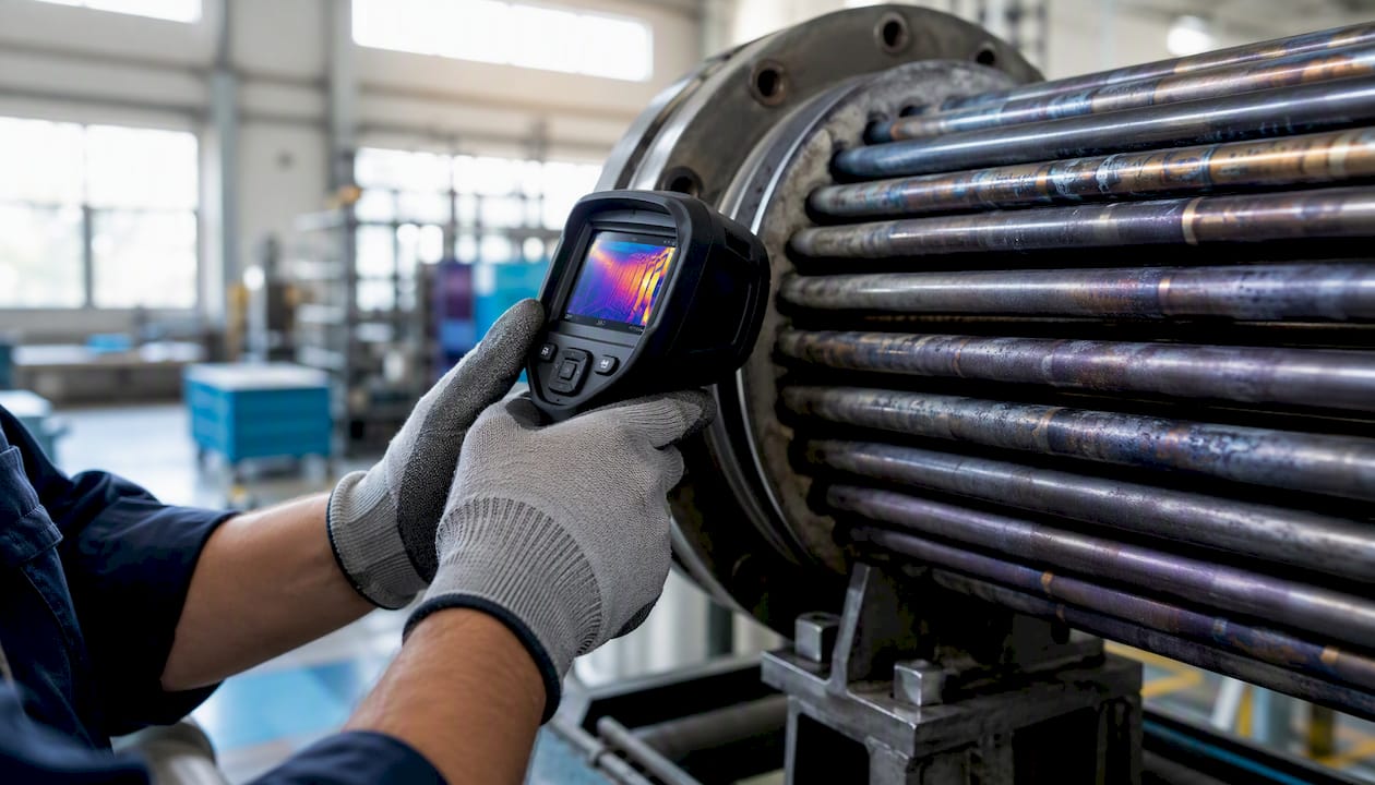
Heat exchanger effectiveness (ε) is the ratio of actual heat transfer to the maximum thermodynamically possible heat transfer between two streams. Once you have ε, the working formula is straightforward: Q = ε · C_min · (T_h,in − T_c,in), where Q_max = C_min · (T_h,in − T_c,in) represents what a counterflow exchanger of infinite area would achieve. Faith A. Morrison’s Michigan Tech lecture notes define this relationship precisely and show why it eliminates the iterative temperature guessing that LMTD requires.
Effectiveness always falls between 0 and 1. The exchanger delivers a high proportion of the theoretical maximum heat transfer. You cannot exceed 1.0 physically; if your calculation returns ε > 1, there is a unit error or a misidentified C_min somewhere.
Method choice in one sentence: use the NTU method when outlet temperatures are unknown and you know UA (or exchanger geometry); use LMTD when both inlet and outlet temperatures are already known and you are sizing or rating from a known temperature program.
Table of Contents
What are the core variables you need for effectiveness calculations?
Before any formula makes sense, the symbols need to be pinned down. The table below maps every variable used throughout this guide.
Symbol | Meaning | Typical Units |
ṁ | Mass flow rate | kg/s or lb/s |
c_p | Specific heat at constant pressure | J/(kg·K) or BTU/(lb·°F) |
Ċ = ṁ·c_p | Heat-capacity rate | W/K or BTU/(hr·°F) |
C_min | Smaller of the two heat-capacity rates | W/K |
C_max | Larger of the two heat-capacity rates | W/K |
C_r | Heat-capacity ratio = C_min / C_max | Dimensionless (0 ≤ C_r ≤ 1) |
Q_max | Maximum possible heat transfer | W or BTU/hr |
U | Overall heat-transfer coefficient | W/(m²·K) or BTU/(hr·ft²·°F) |
A | Heat-transfer area | m² or ft² |
UA | Overall conductance | W/K |
NTU | Number of Transfer Units = UA / C_min | Dimensionless |
ε | Effectiveness = Q_actual / Q_max | Dimensionless (0 ≤ ε ≤ 1) |
Heat-capacity rate is the product ṁ·c_p. It tells you how much energy a stream gains or loses per degree of temperature change. The stream with the smaller Ċ changes temperature more steeply for the same Q, so it sets the thermodynamic ceiling.
Q_max is what you would extract if the stream with C_min underwent the full inlet-to-inlet temperature difference: Q_max = C_min · (T_h,in − T_c,in). This is the ideal counterflow, infinite-area limit. The heat-capacity ratio C_r = C_min / C_max ranges from 0 (one stream is condensing or evaporating, so its temperature stays constant) to 1 (perfectly balanced streams).
NTU = UA / C_min is the dimensionless measure of how much heat-transfer capacity the exchanger has relative to the stream that changes temperature most. A low NTU (say, 0.5) means the exchanger is undersized for the duty; NTU above 3 or 4 puts you well into diminishing-returns territory for most configurations.
Standard assumptions for the closed-form effectiveness relations:
Steady-state operation with no heat loss to surroundings
Constant fluid properties (ṁ, c_p, U) throughout the exchanger
Single-pass geometry or a specified multi-pass arrangement
Specified mixing condition for crossflow (both unmixed, one mixed, or both mixed)
No axial conduction along the wall
These assumptions hold well for most liquid-liquid and gas-liquid exchangers in preliminary design. When properties vary significantly with temperature (high-viscosity oils, near-critical fluids), you need a segmented or numerical approach.
How do the NTU effectiveness relations work for each flow arrangement?
The NTU method gives closed-form expressions for ε as a function of NTU and C_r for every standard flow arrangement. The algebraic origin is the same in each case: write energy balances on a differential element, nondimensionalize temperatures, integrate along the flow path, and apply boundary conditions. The result is always ε = f(NTU, C_r), with the specific function depending on how the streams are arranged.
Counterflow
$$\varepsilon = \frac{1 - \exp[-\text{NTU}(1 - C_r)]}{1 - C_r \cdot \exp[-\text{NTU}(1 - C_r)]} \quad (C_r < 1)$$
For the balanced case C_r = 1:
$$\varepsilon = \frac{\text{NTU}}{1 + \text{NTU}}$$
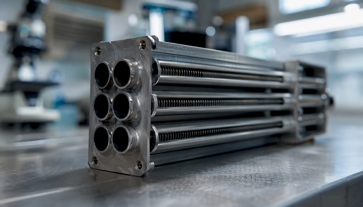
Counterflow consistently delivers higher effectiveness than parallel flow for the same NTU and C_r. Physically, the cold outlet faces the hot inlet, so the driving temperature difference is spread more evenly along the exchanger length. Under the right conditions, the cold-stream outlet temperature can actually exceed the hot-stream outlet temperature, something parallel flow can never achieve.
Parallel flow
$$\varepsilon = \frac{1 - \exp[-\text{NTU}(1 + C_r)]}{1 + C_r}$$
Parallel flow converges to a finite maximum effectiveness even as NTU → ∞: ε_max = 1/(1 + C_r). For C_r = 1, that ceiling is 0.5. Engineers Edge explains that parallel flow is sometimes deliberately chosen despite lower ε, particularly in food processing or pharmaceutical applications where thermal shock to a sensitive product must be avoided by keeping both streams at similar temperatures throughout.
Special case: C_r = 0 (condensers, evaporators)
When one stream undergoes phase change, its temperature stays constant and C_max → ∞, so C_r = 0. Both counterflow and parallel-flow formulas collapse to the same expression:
$$\varepsilon = 1 - e^{-\text{NTU}}$$
This is the simplest and most commonly used single-parameter relation in heat exchanger work.
Crossflow (both streams unmixed)
$$\varepsilon \approx 1 - \exp!\left[\frac{\text{NTU}^{0.22}}{C_r}\left(\exp(-C_r \cdot \text{NTU}^{0.78}) - 1\right)\right]$$
This approximation, widely reproduced in textbooks and university lecture notes, is accurate for most practical NTU ranges. When one stream is mixed and the other is unmixed, a different closed-form applies; the choice of mixing condition must match the physical geometry (finned plate-fin exchangers are typically both-unmixed; shell-and-tube crossflow passes are often one-mixed).
Shell-and-tube 1-2 (one shell pass, two tube passes)
$$\varepsilon = 2\left{1 + C_r + \sqrt{1+C_r^2}\cdot\frac{1+\exp[-\text{NTU}\sqrt{1+C_r^2}]}{1-\exp[-\text{NTU}\sqrt{1+C_r^2}]}\right}^{-1}$$
This is the standard approximation for a 1-2 shell-and-tube exchanger. For more passes, the relation is applied iteratively or replaced by the F-factor correction on LMTD.
Numerical inversion: most of these relations can be inverted analytically for NTU given ε and C_r (counterflow and parallel flow invert cleanly). Crossflow and multi-pass forms often require simple root-finding. A bisection or Newton-Raphson loop converges in fewer than ten iterations for any physically meaningful ε. M. Subramanian’s lecture notes provide stepwise solution patterns that are easy to implement in a spreadsheet or script.
When should you use LMTD instead of the NTU method?
The NTU effectiveness method is the right tool when outlet temperatures are unknown and you know UA (or exchanger geometry). LMTD is easier when you already know all four terminal temperatures and want to find the required UA or area directly.
Iterative LMTD procedure
When outlet temperatures are not fully known but you want to use LMTD (for example, to apply an F-factor chart for a shell-and-tube exchanger), the procedure is:
Guess one unknown outlet temperature based on an energy balance.
Compute both terminal temperature differences: ΔT_1 = T_h,in − T_c,out and ΔT_2 = T_h,out − T_c,in for counterflow (reverse for parallel flow).
Calculate ΔT_lm = (ΔT_1 − ΔT_2) / ln(ΔT_1 / ΔT_2).
Compute Q = U · A · F · ΔT_lm, where F is the correction factor for non-counterflow geometries.
Check Q against the energy balance Q = Ċ_h · (T_h,in − T_h,out) = Ċ_c · (T_c,out − T_c,in).
Update the guessed outlet temperature and repeat until Q converges (typically 3–5 iterations).
The correction factor F accounts for the departure from pure counterflow in shell-and-tube and crossflow exchangers. F-charts are published in Incropera & DeWitt (Fundamentals of Heat and Mass Transfer), TEMA standards, and most heat-transfer textbooks. F drops below 1 whenever the geometry is not pure counterflow; a value of F < 0.75 usually signals that you should add a shell pass rather than increase area.
NTU vs LMTD: when each wins
Use NTU when:
Outlet temperatures are unknown (performance rating of an existing exchanger)
You want to avoid iteration entirely
You are doing parametric studies varying UA or mass flow
Use LMTD when:
All four terminal temperatures are specified (design from a temperature program)
You need to apply F-factor charts for multi-pass shell-and-tube
You are verifying a design against a process specification
One practical note: always carry consistent units through the entire calculation. Mixing BTU/hr with watts, or °F with °C, is the single most common source of nonsensical results. A quick dimensional check on UA (W/K or BTU/hr·°F) before plugging into any formula takes ten seconds and saves hours of debugging.
Worked examples: computing ε, Q, and outlet temperatures
Example 1: Counterflow, C_r < 1
Given:
Hot stream: ṁ_h = 2.0 kg/s, c_p,h = 4,000 J/(kg·K), T_h,in = 90°C
Cold stream: ṁ_c = 1.5 kg/s, c_p,c = 4,200 J/(kg·K), T_c,in = 20°C
UA = 6,000 W/K
Step 1: Compute heat-capacity rates.
Ċ_h = 2.0 × 4,000 = 8,000 W/K
Ċ_c = 1.5 × 4,200 = 6,300 W/K
C_min = 6,300 W/K (cold stream), C_max = 8,000 W/K
C_r is the ratio of the smaller to the larger heat-capacity rate.
Step 2: Compute NTU.
NTU is the ratio of UA to the smaller heat-capacity rate.
Step 3: Apply counterflow ε relation.
ε = [1 − exp(−0.952 × (1 − 0.7875))] / [1 − 0.7875 × exp(−0.952 × (1 − 0.7875))]
Exponent: −0.952 × 0.2125 = −0.2023
exp(−0.2023) = 0.8168
Numerator: 1 − 0.8168 = 0.1832
Denominator: 1 − 0.7875 × 0.8168 = 1 − 0.6432 = 0.3568
ε = 0.1832 / 0.3568 = 0.513
Step 4: Compute Q.
Q_max = C_min × (T_h,in − T_c,in) = 6,300 × (90 − 20) = 441,000 W
Q is calculated by multiplying effectiveness and maximum possible heat transfer.
Step 5: Outlet temperatures.
T_c,out = T_c,in + Q / Ċ_c = 20 + 226,233 / 6,300 = 20 + 35.9 = 55.9°C
T_h,out = T_h,in − Q / Ċ_h = 90 − 226,233 / 8,000 = 90 − 28.3 = 61.7°C
Verification: Energy balance closure: Ċ_h × (90 − 61.7) = 8,000 × 28.3 = 226,400 W. The small rounding difference (≈ 0.07%) confirms the calculation is consistent.
Notice that T_c,out (55.9°C) is below T_h,out (61.7°C), which is physically correct for counterflow at this NTU. For a much higher NTU, the cold outlet would approach the hot inlet temperature.
Example 2: Parallel flow, same inputs
Using identical stream data and UA, but now parallel flow:
Step 1: C_min, C_max, C_r, and NTU are unchanged: C_r = 0.7875, NTU = 0.952.
Step 2: Apply parallel-flow ε relation.
ε = [1 − exp(−NTU × (1 + C_r))] / (1 + C_r)
Exponent: −0.952 × (1 + 0.7875) = −0.952 × 1.7875 = −1.7017
exp(−1.7017) = 0.1824
Numerator: 1 − 0.1824 = 0.8176
Denominator: 1 + 0.7875 = 1.7875
ε = 0.8176 / 1.7875 = 0.457
Step 3: Q and outlet temperatures.
Q is calculated by multiplying effectiveness and maximum possible heat transfer.
T_c,out = 20 + 201,537 / 6,300 = 20 + 32.0 = 52.0°C
T_h,out = 90 − 201,537 / 8,000 = 90 − 25.2 = 64.8°C
The parallel-flow exchanger transfers about 11% less heat than the counterflow arrangement for the same UA and stream conditions. The cold outlet (52.0°C) cannot exceed the hot outlet (64.8°C), which is the fundamental thermodynamic constraint of parallel flow. As NTU → ∞, parallel-flow ε approaches 1/(1 + C_r) = 1/1.7875 = 0.559, a hard ceiling that counterflow does not share. For practical worked examples that extend these calculations to multi-stream and phase-change scenarios, the Jewlztech engineering blog covers additional configurations.
Special case: C_r = 0 (phase change)
If the hot stream is condensing steam (T_h = constant = 120°C), C_max → ∞ and C_r = 0. With NTU = 0.952:
ε is calculated from the special case formula for phase change with given NTU.
Both counterflow and parallel-flow give the same result. The condensing side imposes no capacity-rate constraint, so flow arrangement is irrelevant to effectiveness.
Numerical solving when closed form is not directly invertible
If you need NTU given ε = 0.70 and C_r = 0.5 for crossflow (both unmixed), the crossflow formula cannot be cleanly inverted. Set up f(NTU) = ε(NTU, 0.5) − 0.70 = 0 and apply bisection between NTU = 0.5 and NTU = 3.0. Three to five iterations resolve NTU to within 0.01. The Elysia Tools NTU calculator handles this numerically and supports parallel, counterflow, shell-and-tube 1-2, and crossflow unmixed configurations, making it a fast verification check for hand calculations.
How do ε vs NTU charts guide your design decisions?
The canonical ε vs NTU curves show one consistent pattern: effectiveness rises steeply at low NTU, then flattens as NTU increases. Adding area beyond NTU ≈ 3–4 yields diminishing returns for most C_r values. This is the core design insight the charts communicate.
Reference table: ε at common NTU and C_r values (counterflow)
The values below come from the closed-form counterflow relation and tabulated effectiveness data in standard university references.
NTU | C_r = 0 | — | — | C_r = 0.75 | C_r = 1.0 |
3.0 | — | — | — | 0.848 | 0.750 |
4.0 | 0.982 | 0.957 | 0.929 | 0.900 | 0.800 |
At C_r = 0 (phase change), ε = 1 − e^(−NTU), so the curve rises fastest. At C_r = 1 (balanced streams), the counterflow formula gives ε = NTU/(1 + NTU), which grows more slowly. Parallel-flow curves are always below the counterflow curves for the same C_r, and they plateau at 1/(1 + C_r).
Translating an ε target into UA and area
Once you have a target effectiveness, the path to hardware is:
Read NTU from the table (or compute it from the inverted formula).
UA = NTU × C_min.
A = UA / U, where U is the overall heat-transfer coefficient for your fluid pair and surface geometry.
Realistic U ranges: liquid-liquid exchangers typically run 500–2,000 W/(m²·K); gas-gas exchangers often fall in the 25–250 W/(m²·K) range; condensers and evaporators can reach 1,000–6,000 W/(m²·K) depending on fluid and surface enhancement. These ranges are wide enough that a factor-of-two uncertainty in U translates directly into a factor-of-two uncertainty in required area, which is why fouling factors matter so much at the sizing stage.
The “10-13 rule” does not exist
No universally accepted “10-13 rule” for heat exchanger effectiveness exists in the engineering literature. The phrase circulates informally in some classroom settings, but it has no thermodynamic basis and no standard definition. Relying on it instead of computing ε from the NTU method is the kind of shortcut that produces designs that are either oversized by 40% or undersized and failing within a year. Calculate; do not guess.
How fouling reduces effectiveness in practice
Fouling deposits on heat-transfer surfaces increase thermal resistance, reduce the effective U, and therefore reduce UA and NTU for a fixed geometry. A fouled exchanger operating at the same flow conditions as a clean one will show lower outlet temperatures on the cold side and higher outlet temperatures on the hot side. Monitoring the ratio of actual Q to design Q over time is a practical way to track fouling progression without disassembling the unit.
A short checklist for accounting for real-world factors in preliminary sizing:
Apply TEMA fouling resistances for both streams from the start
Add a 10–15% area margin on top of the clean-UA calculation
Check whether partial phase change (subcooled condensate, superheated vapor) changes the effective C_r along the exchanger length
Verify that maldistribution (uneven flow across parallel channels) is not reducing effective area; this is common in plate heat exchangers with poorly designed headers
If bypass flows are possible (shell-side bypasses in shell-and-tube), account for them with a bypass fraction correction on the shell-side coefficient
Pro Tip: Run a two-point NTU sensitivity check on every design: compute ε at 80% and 120% of your design UA. If ε changes by more than 0.05 between those two points, you are on the steep part of the curve and the design is sensitive to manufacturing tolerances or fouling. If ε barely moves, you are in the flat region and can likely reduce area without sacrificing performance.
How do you compute effectiveness efficiently in practice?
Manual calculation works for a single design point. For parametric studies, sensitivity analyses, or designs with variable fluid properties, a structured computational workflow saves significant time and reduces transcription errors.
MATLAB or EES approach
In MATLAB, define a function epsilon_cf(NTU, Cr) that returns the counterflow ε, then call it inside a loop over a UA vector. For crossflow inversion, fzero(@(NTU) epsilon_crossflow(NTU, Cr) - target_eps, [0.1, 10]) converges reliably. EES (Engineering Equation Solver) handles the implicit relations directly without manual root-finding, which makes it particularly convenient for multi-stream or multi-pass configurations.
For geometry preparation and exchanger area calculations, a CAD viewer can help engineers extract surface areas from exchanger geometry before feeding them into thermal calculations.
Key Takeaways
Heat exchanger effectiveness (ε) is the single most useful dimensionless metric for both rating an existing exchanger and sizing a new one, because it directly connects UA, stream capacity rates, and achievable outlet temperatures without iteration.
Point | Details |
ε definition and formula | ε = Q_actual / Q_max; compute Q = ε · C_min · (T_h,in − T_c,in) once ε is known. |
NTU vs LMTD choice | Use NTU when outlet temperatures are unknown; use LMTD when all four terminal temperatures are specified. |
Counterflow vs parallel flow | Counterflow always yields higher ε for the same NTU and C_r; parallel flow caps at ε_max = 1/(1 + C_r). |
Design translation | UA = NTU · C_min; then A = UA / U using realistic U for your fluid pair and surface geometry. |
Jewlztech Thermalysis Toolkit | Handles variable properties, multiple flow arrangements, and fouling scenarios in an Excel-based workflow for repeatable engineering calculations. |
Why the classroom-to-field gap in heat exchanger work is wider than it looks
Most undergraduate courses teach the NTU method cleanly: fixed properties, neat numbers, one flow arrangement. The formulas close, the answer matches the back of the book, and the student moves on. The gap opens the moment a real exchanger enters the picture.
Real exchangers have fouled surfaces, maldistributed flow, and fluid properties that shift across a 200°C temperature range. The closed-form ε relations are still the right starting point, but they are the beginning of the analysis, not the end. An engineer who treats a textbook ε value as a final answer without checking fouling factors, verifying the mixing-condition assumption, or running a sensitivity on UA is building on a foundation that will crack under operating conditions.
The other thing courses underemphasize is the C_min identification step. It sounds trivial, but on a real project with multiple streams, phase changes, and variable c_p, getting C_min wrong propagates through every downstream calculation. The verification step, checking that Q computed from the hot side matches Q computed from the cold side, takes thirty seconds and catches this class of error immediately.
One practical tip for students and early-career engineers: start every new exchanger design with conservative fouling factors (use TEMA values, not optimistic clean-surface assumptions) and run the two-point NTU sensitivity described in the pitfalls section. If the design is robust to a 20% reduction in UA, it will survive the first year of operation. If it is not, you want to know that at the design stage, not during a plant shutdown.

The Thermalysis Toolkit handles the calculations this guide just walked you through
Engineers who work through the NTU method by hand understand what the formulas are doing. The Thermalysis Toolkit from Jewlztech is where that understanding meets production-grade calculation.

The toolkit covers the full workflow: enter your stream conditions, select a flow arrangement, and get ε, NTU, Q, and outlet temperatures in one pass, with the property database handling variable c_p so you are not locked into constant-property assumptions. Fouling scenarios, UA sensitivity sweeps, and multi-arrangement comparisons are built into the interface and export directly to Excel for documentation.
What it gives you directly:
Variable-property calculations across a wide temperature range using a built-in fluid database
NTU and LMTD calculation modes for both rating and sizing problems
Exportable Excel-based reports ready for design reviews or academic submissions
Visit the Thermalysis Toolkit product page to download the toolkit and run your first ε/NTU calculation today.
Useful sources for heat exchanger effectiveness
These references cover derivations, worked examples, charts, and calculators. Each is annotated so you can go directly to the material you need.
Faith A. Morrison, Michigan Tech lecture notes — Defines ε precisely, derives Q = ε · C_min · (T_h,in − T_c,in), and motivates the NTU approach as an alternative to iterative LMTD. Good starting point for students.
NTU method (Wikipedia) — Provides the complete set of canonical ε(NTU, C_r) formulas for parallel flow, counterflow, crossflow, and special cases. Useful as a quick formula reference.
M. Subramanian lecture notes, IIT Madras — Stepwise derivations and worked arithmetic examples for both cocurrent and countercurrent cases. Particularly useful for verifying hand calculations and understanding the derivation structure.
Effectiveness-NTU tables and relations, University of Mosul lecture notes — Tabulated effectiveness relations and plotted curves for shell-and-tube, double-pipe, and crossflow configurations. Use these for the ε vs NTU reference charts.
Engineers Edge: parallel and counterflow design considerations — Explains the thermodynamic and process reasons for choosing counterflow vs parallel flow, including cases where parallel flow is preferred despite lower effectiveness.
Thermal Engineering: NTU effectiveness method — Concise method comparison between NTU and LMTD, with practical guidance on when each approach is appropriate.
Elysia Tools NTU calculator — Online calculator implementing closed-form NTU relations for parallel, counterflow, shell-and-tube 1-2, and crossflow unmixed. Useful for numerical verification of hand calculations.
Thermalysis Toolkit, Jewlztech — Excel-based engineering toolkit with variable-property support, NTU/LMTD calculators, and exportable sensitivity analyses. The software option for engineers who need repeatable, documented calculations beyond single design points.
Recommended
Comments