
5 Step Fan Curve Selection for Engineers With Simulation Checks

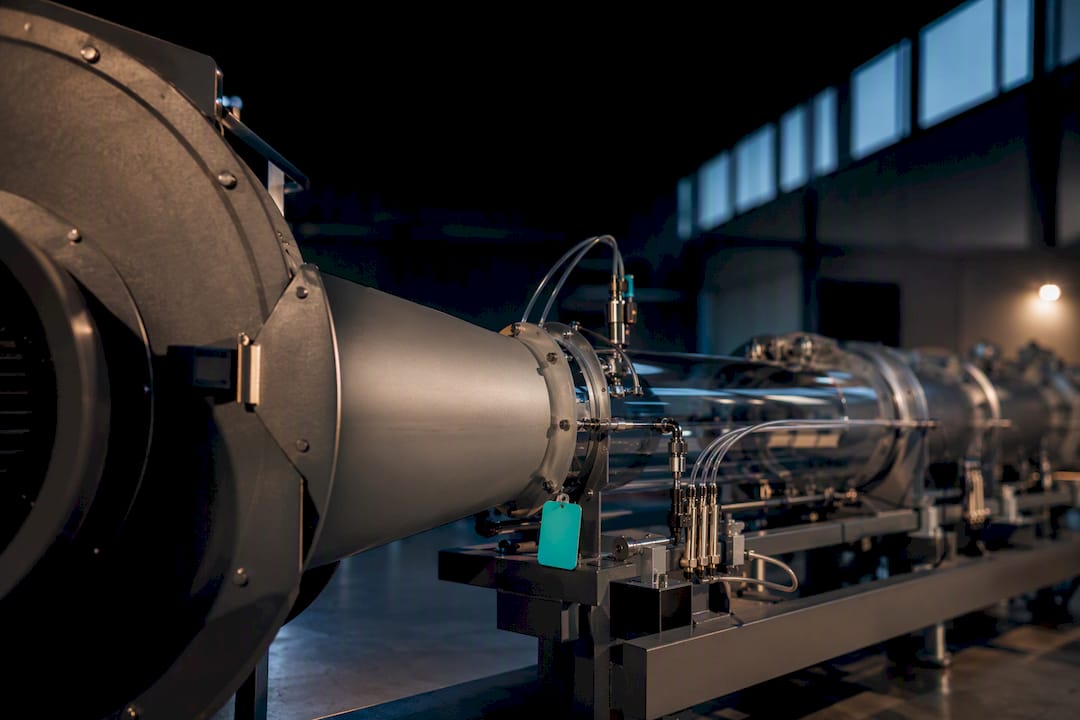
Everything else in fan curve selection, from computing system resistance to choosing between forward-curved and airfoil blades, exists to help you hit that one target reliably.
TL;DR:
Maintaining a fan within ±10% of the Best Efficiency Point minimizes energy waste and mechanical issues, with around 15% stall margin recommended for vaneaxial fans to prevent flow separation.
The actual operating point depends on the intersection of the fan and system curves; changes in ductwork, filters, or dampers can shift this point significantly.
Correcting manufacturer fan curves for site conditions like altitude or temperature is essential; uncorrected data can lead to inaccurate performance expectations.
Variations in fan type, such as forward-curved or backward-curved, influence curve shape and overload risks, affecting system efficiency and motor sizing.
CFD and reduced-order models are valuable for complex inlet geometries or tight spaces, offering predictions within approximately 7% accuracy beyond manual curve matching.
Table of Contents
What a Fan Curve Actually Shows You
A fan curve plots airflow (CFM or m3/s) against pressure (inches of water gauge or Pascals), usually as static pressure unless the chart says otherwise. Total pressure and static pressure are not interchangeable, and confusing them is one of the more common ways engineers misread a rating sheet.
To use the curve correctly, find your required flow on the horizontal axis, trace up to the pressure curve, then project across to the brake horsepower and efficiency curves plotted on the same chart. That single vertical line gives you pressure, power draw, and efficiency at once, which is exactly how AMCA describes the standard reading method. Manufacturers publish these curves at a specific air density and test speed, so any deviation in altitude, temperature, or actual fan speed requires a correction before the numbers mean anything for your site. Skip that step and you’re comparing your system to a fan that doesn’t quite exist in your building.
Reading BEP, Stall, and the Power Curve Correctly
Best Efficiency Point (BEP) is the flow and pressure combination where the fan converts the most input power into useful airflow. Selecting outside that zone doesn’t just waste energy. It changes how the fan behaves mechanically.
Practical guidance from AMCA and ASHRAE targets operation within ±10% of BEP, with ±10% to 20% considered acceptable in most applications. Push further left and you enter the stall region, where flow separates from the blades and the pressure curve flattens or dips unpredictably.
Watch for these signals when evaluating a curve:
A flattening or reversing slope on the pressure curve as flow drops, which signals the onset of stall
Rising vibration or a noticeable roar at low-flow, high-pressure operating points
A brake horsepower curve that keeps climbing as flow decreases (an overloading curve) versus one that peaks and falls off (non-overloading)
Stall margin guidance: vaneaxial fans typically need 15% to 20% clearance from the stall region to avoid flow separation and vibration, according to selection guidance from the Industrial Engineering Studio. Overloading power curves matter for motor sizing. If BHP keeps rising as static pressure increases beyond design, an undersized motor will trip or burn out under upset conditions, not just at the design point.
Finding the Real Operating Point on the System Curve
The fan curve only tells half the story. Your actual operating point is wherever the fan curve crosses the system curve, and the system curve is a function of resistance, not fan selection.
System resistance follows the relationship ΔP = K·Q², where K is a constant you calculate from a known design condition. Here’s the practical sequence:
Sum every pressure drop in the system at design airflow: ductwork, elbows, dampers, filters, coils, and terminal devices.
Back out K using K = ΔP / Q² from that known design point.
Generate the system curve by recalculating ΔP across a range of flows using that same K.
Overlay it on the fan curve. The intersection is your real operating point, not the point printed on the fan’s nameplate.
That intersection moves whenever the system changes. A clogged filter raises K and shifts the operating point left, toward lower flow and higher pressure. Adding ductwork or opening a damper does the opposite. This is why the curve you plot during design is a snapshot, not a guarantee.
Pro Tip: Always verify the assumed operating point during testing, adjusting, and balancing (TAB). Field measurements routinely show 10% to 15% deviation from calculated K values because as-built ductwork rarely matches the drawings exactly.
A Step-by-Step Workflow for Selecting the Right Fan
Fan sizing guidelines boil down to five sequential steps, and skipping the order is where most selection errors creep in.
Confirm design airflow. Start with the calculated ventilation or process requirement, then add margin for future load growth or field variability. Ten percent is a common starting allowance, though process-critical systems may need more.
Calculate system pressure and K. Sum every component’s pressure drop at design flow, including a 10% to 15% field allowance for installation imperfections that the Enginist selection methodology recommends building into any system curve.
Pull manufacturer curves at the intended operating speed and air density. If your site density differs from the test condition (altitude, elevated temperature), correct the curve before comparing it to your system curve.
Plot the system curve on the candidate fan curves and check the intersection. Confirm the operating point sits near BEP, verify stall margin, and check that BHP stays under the motor’s rated capacity. If it doesn’t clear all three checks, go back to the manufacturer’s selection chart and try another model or size.
Size the motor with appropriate service factor, and if you’re using a variable frequency drive, confirm the motor and drive are rated compatible across the intended speed range.
Before you finalize anything, run these final checks:
How does the fan behave at off-design conditions, like a partially closed damper or a bypassed zone?
What happens to the operating point with a dirty filter at end-of-life pressure drop?
Does the selection meet sound criteria at the actual operating point, not just at the rated point?
Have you applied inlet and discharge system-effect corrections for duct connections that don’t match the test setup?
How Fan Type Changes the Curve You’re Working With
Fan sizing isn’t just about matching a number. Fan type dictates the curve shape you’re negotiating with, and that shape determines how forgiving the fan is if your system calculations are slightly off.
Forward-curved fans produce a relatively flat pressure curve and compact footprint, common in residential and light commercial equipment. Their power curve is overloading, meaning BHP keeps rising as pressure increases past design, which creates real motor-overload risk if the system resistance ends up higher than calculated.
Backward-curved and airfoil fans have steep, non-overloading power curves and typically deliver the highest efficiency of any centrifugal type. They dominate air handling units and any application where efficiency is a design priority, since BHP peaks and then falls rather than climbing indefinitely.
Radial fans are the workhorses for particulate-laden or abrasive airstreams. They sacrifice some efficiency for mechanical ruggedness at higher pressures, which is why you see them in material handling and dust collection.
Axial and vaneaxial fans move large volumes at low to medium pressure efficiently, but their curves carry a pronounced stall region on the left side. Selection margin against that stall zone matters more here than with any centrifugal type.
Using Fan Laws to Shift Curves for Speed Control
The affinity laws describe how a fan’s curve moves when you change speed: flow scales directly with speed (Q ∝ N), pressure scales with speed squared (P ∝ N²), and power scales with speed cubed (Power ∝ N³).
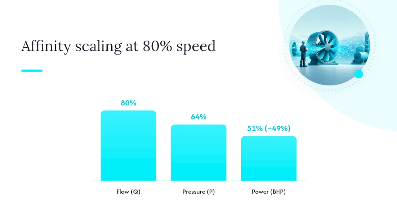
That cubic relationship is why variable frequency drives deliver outsized energy savings. Cut fan speed by 20% and power draw drops by roughly 49%, a return on a fairly small speed reduction that throttling dampers can never match. Generate a shifted curve by scaling flow and pressure at each point using the ratio of new speed to rated speed, then recheck BHP at reduced speed. VFD control shifts the entire curve rather than restricting airflow at a fixed speed, which is why it beats throttling for efficiency. Set a minimum safe operating speed so control sequences never push the fan back into stall as speed drops.
Verification Checklist and Pitfalls That Trip Up Even Experienced Engineers
Motor sizing needs to account for the fan’s power curve type. Overloading fans (most forward-curved models) need service factor margin above the calculated BHP at the worst-case operating condition, not just at design.
Density correction matters more than most selection sheets admit. A fan rated at sea level, standard temperature will deliver less mass flow at altitude or in a hot equipment room, even though the volumetric CFM reading looks unchanged.
Common mistakes worth flagging before they become field problems:
Assuming the catalog duty point equals installed performance, when inlet and discharge system effects routinely add unaccounted resistance
Ignoring dirty-filter pressure drop and sizing only for clean-filter conditions
Undersizing the motor for off-design states like a bypassed zone or a stuck damper
Pro Tip: Request the manufacturer’s system-effect factor for your specific inlet and discharge configuration. Elbows close to the fan inlet can add 10% or more to effective resistance that a clean-duct calculation misses entirely.
When Simulation Beats Manual Curve Matching
Manual curve matching handles most jobs fine. Complex inlet geometry, tight enclosures, or electronics cooling applications with dense component stacking are where it starts to break down, because installed performance can diverge meaningfully from the published curve.
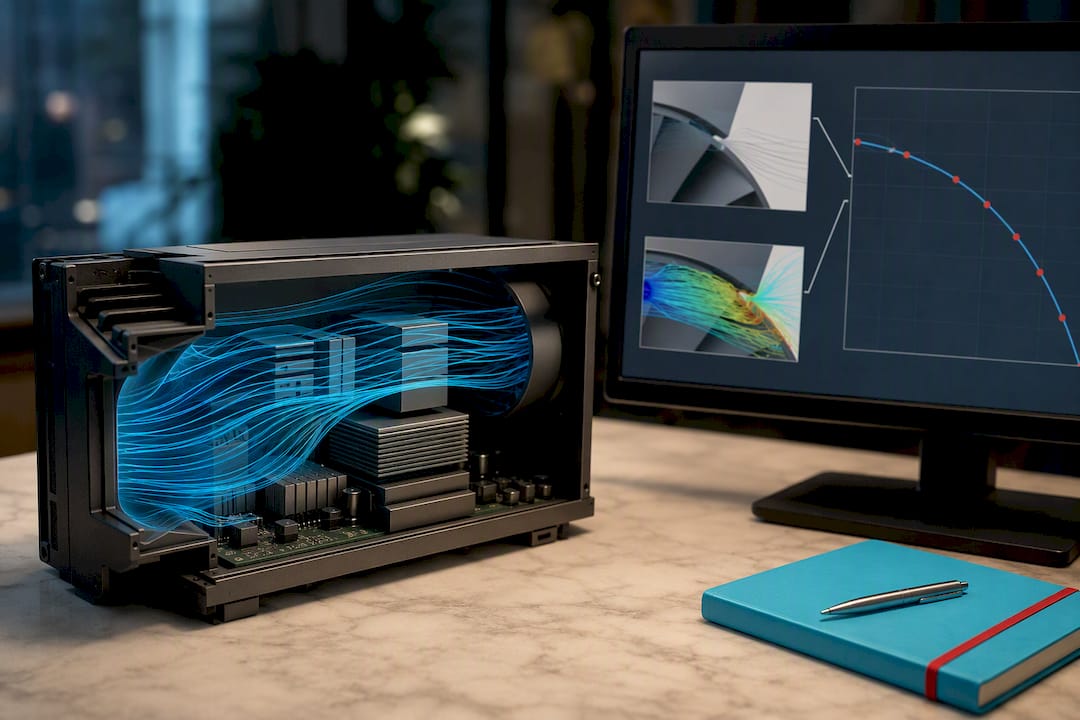
Reduced-order and CFD-validated models can predict installed pressure-flow curves within roughly 7% error in nominal operating regions, capturing effects like tip clearance and inlet distortion that a flat catalog curve can’t show. Tip clearance alone can swing efficiency by several percent on small axial fans. A practical workflow: do the manual curve match first, and reach for simulation only when your BEP margin is thin or the inlet/discharge geometry is unusual enough to worry you. Engineers working through electronics cooling layouts often lean on CFD templates built for that exact problem rather than building a model from scratch.
What Field Experience Teaches About Fan Selection
Efficiency-optimized curves look great on paper until a tenant swaps out filters for a denser MERV rating, or a future renovation adds ductwork nobody modeled. I’d rather see an engineer accept a slightly lower BEP match for a fan with a forgiving, non-overloading power curve than chase the last percentage point of efficiency on a system with real uncertainty. When a selection sits close to any boundary, whether that’s stall margin or BHP headroom, validate it with simulation or commissioning data before you commit.
— Joel
Validate Tight Selections Before They Become Field Problems
When your fan curve selection lands close to a boundary, whether that’s a thin BEP margin, an unusual inlet configuration, or a dense electronics enclosure, guessing costs more than checking. Downloadable thermal and CFD templates let you run installed-performance checks and sensitivity studies before the fan gets ordered, not after it’s humming in a duct that doesn’t match the drawing.

The toolkit works alongside your manual curve matching rather than replacing it: use the affinity laws and system curve method to narrow candidates, then run a reduced-order or CFD pass on the borderline cases where inlet distortion, tip clearance, or tight enclosures could shift the real operating point away from what the catalog promises. It’s built for engineers who want a second check on a selection before hardware gets ordered, not a replacement for the fundamentals. Start with the thermal analysis toolkit to see how the templates handle your next borderline selection.
Where to Dig Deeper on Fan Curve Standards
For certified test methods and energy calculations, AMCA’s fan energy index standard lays out the governing methodology manufacturers use to rate published curves. Clarage’s “Understanding Fan Curves” application note offers worked examples that pair well with the reading technique covered above.
Sources
FAQ
What Is a Fan Curve in Simple Terms?
A fan curve is a manufacturer chart plotting airflow against pressure for a specific fan at a given speed and air density, with power and efficiency curves typically overlaid on the same chart.
How Close to BEP Should a Fan Operating Point Be?
Aim within 10% of best efficiency point, with 10% to 20% deviation generally acceptable per AMCA and ASHRAE guidance; operating further off BEP raises energy cost and stall risk.
What Happens if a Fan Operates in the Stall Region?
Flow separates from the blades, pressure output becomes unstable, and vibration and noise increase; vaneaxial fans typically need 15% to 20% stall margin to avoid this.
How Do Affinity Laws Apply to Fan Speed Control?
Flow scales linearly with speed, pressure scales with speed squared, and power scales with speed cubed, so a 20% speed reduction cuts power by roughly 49%, making VFDs highly effective for energy savings.
When Should an Engineer Use CFD Instead of a Manual Fan Curve?
Reach for simulation when BEP margin is thin, inlet or discharge geometry is unusual, or the application involves dense electronics cooling, since reduced-order models can predict installed curves within roughly 7% error in nominal operating regions.
Recommended
Comments