
Stop Wasting Weeks: 3 Electronics Cooling CFD Templates for Engineers

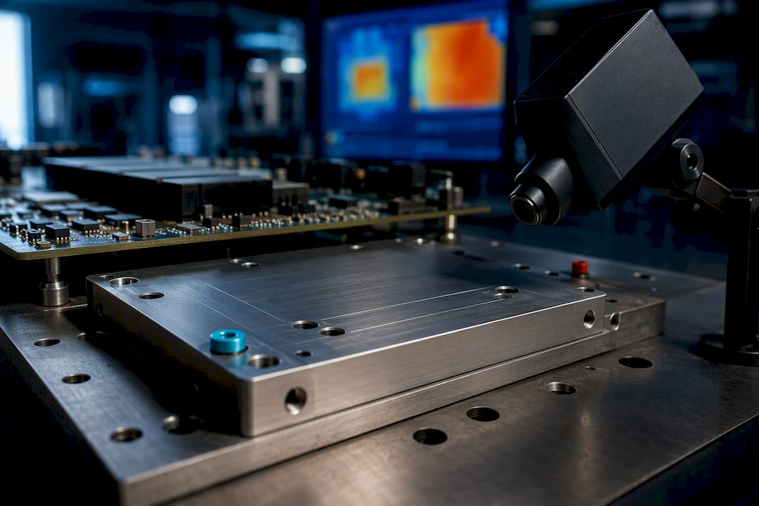
CFD gives you the predictive insight to locate hotspots, quantify thermal resistance chains, and compare cooling routes before you cut metal. Use reduced-order models for fast system-level screening, and full 3D conjugate heat transfer for final verification against hardware. This guide walks through both, with setup checklists, common failure points, and templates you can adapt today.
TL;DR:
Reduced-order models can solve transient electronics thermal problems up to 40,000 times faster than full 3D CFD while maintaining accuracy across varying boundary conditions.
Mesh refinement, realistic boundary conditions, temperature-dependent properties, and proper interface resistance assumptions are critical to building a trustworthy CFD model.
Validating simulations through energy balance checks, correct power mapping, and material property accuracy prevents large errors and ensures reliability.
Full 3D CFD is often needed only for final verification, with ROMs used in early design phases to identify promising options quickly.
Avoid common pitfalls by matching CFD fidelity to the specific question, and treat thermal interface resistance and power mapping as primary suspects when results seem off.
Table of Contents
What Electronics Cooling CFD Actually Models
Electronics cooling CFD is really a stack of coupled physics problems wearing one name. At its core sits conjugate heat transfer (CHT), the method that solves conduction in solids and convection in the surrounding fluid at the same time, rather than treating them as separate problems stitched together with a guessed boundary condition. Conjugate heat transfer is the right call whenever solid-fluid coupling is strong, which in electronics means almost always: a PCB conducting heat laterally through copper planes while air or coolant strips it away convectively is a textbook CHT case.
Layered on top of CHT is electrothermal coupling. Chip power dissipation is temperature-dependent, so a die that runs hotter often draws more leakage current, which raises power, which raises temperature further. Decoupling thermal and electrical analysis throws away that feedback loop, and on tightly packed 2.5D or 3D IC stacks the error compounds fast across device-to-system scales.
You will also need to decide when full geometric detail earns its keep versus when an approximation gets you the same answer faster:
Radiation matters at low air velocities, in vacuum or space-rated enclosures, and for high-emissivity surfaces at elevated temperature; skip it for high-flow forced-air systems where convection dominates by an order of magnitude.
Porous-media approximations replace dense fin arrays or heat sink cores with a permeability and inertial resistance tensor, cutting mesh count dramatically while preserving pressure drop and bulk thermal behavior.
Fidelity escalation should follow the question you’re asking: a first-pass thermal budget tolerates coarse assumptions, but a hotspot verification for a safety-critical junction temperature does not.
The trade-off is always solve time against answer trustworthiness. A full transient CHT run on a populated server chassis can take days on a workstation; a screening study with simplified boundary conditions can run in minutes. Neither is wrong, they just answer different questions.
When Do You Actually Need ROMs Instead of Full CFD?
Running full 3D CFD on every design iteration is how projects miss deadlines. Reduced-order models (ROMs) solve that problem by compressing a validated 3D thermal solution into a fast-executing mathematical surrogate, and the speedup is not incremental.
Boundary-condition independent ROMs (BCI-ROMs) are a specific flavor built to stay accurate even when the operating conditions change after the ROM was generated. A conventional ROM trained at one fan speed and one ambient temperature can drift badly if you change either. A BCI-ROM is constructed so it stays valid across a range of power maps, flow rates, and ambient conditions without rerunning the full 3D model for each case.
The speed gap is not subtle. Reduced-order and BCI-ROM approaches can solve transient electronics thermal problems up to 40,000 times faster than full 3D CFD in representative cases, while retaining predictive accuracy across varying boundary conditions.
A workable multi-fidelity workflow looks like this:
Screening pass: run a ROM across dozens or hundreds of design or operating-point combinations to identify the handful worth deeper study.
Refined 3D study: take the shortlisted candidates and run full CHT with detailed geometry, real material properties, and realistic boundary conditions.
Validation loop: compare the refined CFD result against bench measurement, then feed corrections back into the ROM if it will be reused.
Machine-learning surrogates and physics-informed ML (PIML) models extend this same idea, trading some interpretability for speed on very large design spaces. The catch is verification: a surrogate is only as good as the training data spanned by your actual operating envelope, so extrapolating beyond that range without checking against a real CFD run or hardware test is asking for a confidently wrong answer. The safest posture, and the one worth defaulting to, is using ROMs for exploration and full CHT for final sign-off.
Building a Model You Can Actually Trust: A Setup Checklist
A CFD model is only as good as the assumptions baked into its setup, and most bad results trace back to one of five decisions made in the first hour of building the model.
Simplify geometry deliberately, not lazily. Remove fasteners, small brackets, and cosmetic features that don’t affect flow or heat path. Replace dense fin arrays or complex heat sink cores with a porous-media substitution parameterized from a detailed representative cell, which preserves thermal resistance and flow distribution at a fraction of the mesh cost.
Mesh to the physics, not to a target cell count. Hotspots, thin thermal interface layers, and narrow channel flows all need local refinement. Run a formal mesh-independence check: refine until your junction temperature and pressure drop change by less than roughly 1 to 2 percent between successive mesh levels.
Assign temperature-dependent material properties, not constants. Silicon conductivity, solder, and TIM materials all shift meaningfully across an operating temperature range. Anisotropic conductivity matters for PCB copper planes and for graphite or composite heat spreaders, where in-plane and through-plane conductivity can differ by an order of magnitude.
Set boundary conditions that reflect reality, not convenience. Use actual fan curves rather than a flat velocity inlet, and couple ambient conditions realistically rather than assuming an isolated enclosure with no thermal path to the environment.
Start thermal interface resistance from a sourced value, then test it. A commonly cited starting point for high-performance thermal paste is around 2.5 x 10^-4 m²·K/W. Run the model at that value, then at half and double it, to see how sensitive your junction temperature prediction actually is.
Pro Tip: Build your mesh-independence and TIM sensitivity checks into the model from day one, not as an afterthought once results look “off.” Retrofitting sensitivity studies onto a finished model wastes far more time than building the habit in from the start.
Every one of these steps ties back to the same underlying goal: minimizing the total thermal resistance chain from junction to ambient. CFD’s real value is guiding design changes that shorten that chain across chip, package, and system level, not just producing a pretty color plot.
Validating Your Model and Catching the Errors That Actually Matter
Validation and calibration are not the same activity, and treating them as interchangeable is where a lot of confidence goes wrong. Validation compares your model’s predictions against independent measurement data you did not use to tune anything. Calibration adjusts unknown parameters, TIR being the classic example, until the model matches known measurements. Do calibration first, on a controlled test case, then validate on a separate configuration you have not touched.
Collect the right data before you start: junction or case temperatures at multiple points, actual flow rates rather than nominal fan-curve values, and a real power map instead of a single lumped wattage number.
The recurring sources of large errors are predictable:
Thermal interface resistance gets assumed as perfect contact far too often, which systematically underestimates junction temperature.
Power mapping errors, especially lumping distributed dissipation into a single point source, distort local hotspot predictions even when total power is correct.
Surface emissivity and contact resistance at mechanical interfaces are frequently left at solver defaults that don’t match your actual materials.
Turbulence model limits show up in separated or transitional flows common in electronics enclosures, where a standard k-epsilon model can miss recirculation zones entirely.
A well-run CPU water-block simulation reported an energy balance closure of 99.6 percent at steady state, alongside a thermal resistance result within the expected range. That kind of energy balance check, alongside residual monitoring and a mesh-independence sweep, is the fastest way to catch a model that’s converged numerically but wrong physically.
Run the energy balance every time: total power in should equal total heat rejected out, within a percent or two, before you trust anything else the model tells you.
Modeling High-Flux Active Cooling: Cold Plates, Jets, and Immersion
Passive air cooling runs out of headroom once flux densities climb, and that’s where active cooling routes take over. Liquid cooling, jet impingement, and spray cooling now dominate the research and application landscape for high-heat-flux electronics, and each demands a different modeling strategy.
Microchannels and cold plates: model channels explicitly when channel geometry directly drives your design decision (channel width, fin spacing); switch to a porous-media approximation, parameterized from a detailed sub-model, once you’re studying system-level flow distribution across many parallel channels.
Jet impingement: get the inflow velocity profile right, since impingement heat transfer is extremely sensitive to it, and refine the mesh tightly near the impingement wall where the boundary layer is thinnest. Transient analysis matters if the jet or target moves; steady-state is usually fine for a fixed nozzle array.
Immersion and multiphase cooling: two-phase immersion adds boiling and vapor transport to the problem, which means validating against measured heat transfer coefficients and critical heat flux data becomes non-negotiable rather than optional.
Micro and nanostructured surfaces: these can push performance further, but manufacturing scalability remains a real constraint worth checking before you design around a feature that can’t be fabricated at volume.
The trade-off across all of these is heat removed per unit of auxiliary power. A cold plate that rejects twice the heat of a competing design but demands four times the pump power isn’t necessarily the better system-level choice. Weigh pressure drop, pump or fan power, and long-term reliability, including erosion and fouling risk in liquid loops, alongside the raw thermal number. Before committing to any active loop, it’s worth running the decision framework against a passive alternative to confirm the added complexity earns its keep.
Three Templates You Can Adapt This Week
Building from a known-good template beats starting from a blank geometry every time. Here are three worth keeping on hand.
CPU water-block template: approximate the fin array as a porous zone parameterized from a detailed representative cell, rather than meshing every fin. Typical high-performance water-block thermal resistance lands in a low range once flow rate and TIM are dialed in correctly; a pressure-based steady solver with a k-omega SST turbulence model is a reasonable default starting point.
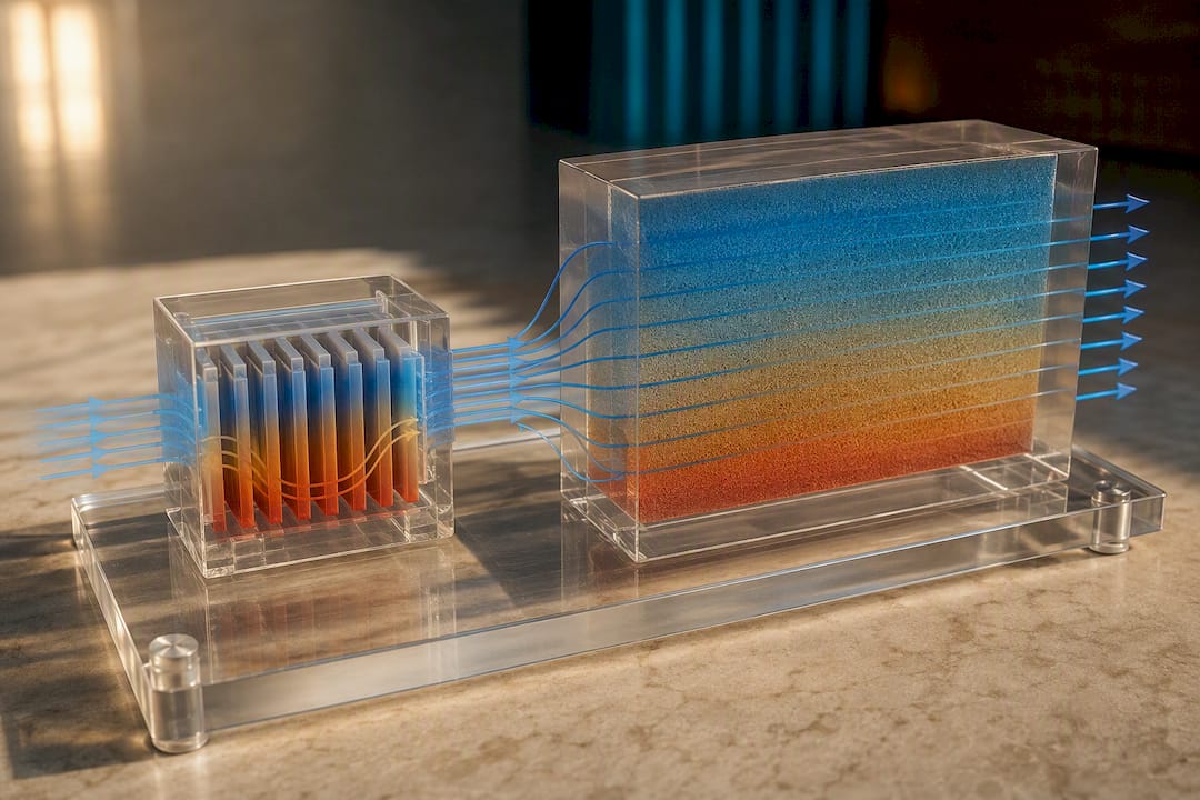
PCB hotspot template: simplify the board stackup into equivalent-conductivity layers instead of modeling every copper trace, then refine the mesh locally around the suspected hotspot component. Expected outputs are junction temperature, local board temperature gradient, and airflow velocity near the component.
Rack-scale ROM template: use a BCI-ROM for transient system-level studies across varying IT load and cooling setpoints, then validate at a handful of operating points against either full CFD or rack-level sensor data.
Template | Primary simplification | Key validation measurement |
CPU water block | Porous-media fin array | Thermal resistance, energy balance |
PCB hotspot | Equivalent-conductivity stackup | Junction temperature, local gradient |
Rack-scale ROM | BCI-ROM surrogate | Transient temperature at sensor points |
Adapting any of these means swapping in your own geometry and boundary conditions while keeping the simplification logic intact, then rerunning the same validation measurements the template calls for. Measure power, flow rate, and at least one point temperature before you touch the mesh.
An Engineer’s View on Building These Tools
Joel has spent years working through electronics thermal management problems where the gap between a clean CFD result and what actually happens on a bench is the whole job. That gap is where Jewlztech’s tools live.
Free CFD and thermal simulation tools let you run the screening pass described above without a license barrier standing between you and a first answer.
The heat exchanger optimization tool applies directly to cold-plate and liquid-loop sizing decisions covered in the active cooling section.
The Thermalysis engineering toolkit covers conduction, convection, and radiation with variable material properties and a built-in property database, useful for the material-property step in the setup checklist above.

Readers working through the templates in this guide can pull material property values, run a first thermal resistance estimate, and check TIM sensitivity, all before opening a full CFD license.
Where Most Engineers Get This Wrong
The conventional advice on electronics cooling CFD treats fidelity as a single dial: turn it up for accuracy, turn it down for speed. That framing is too simple. The real skill is knowing which question you’re answering at each project stage, and matching the tool to it rather than defaulting to whatever CFD setup you used last time.
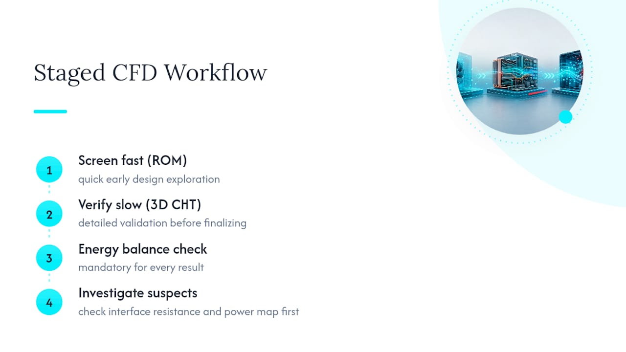
Most teams either over-invest in full 3D CHT for early design exploration, burning weeks on geometry nobody will keep, or under-invest in validation once a “good enough” ROM ships into production. Both mistakes come from skipping the staged workflow: screen fast with a ROM, verify slow with full CHT, and never skip the energy balance check regardless of which tool you used.
If there’s one habit worth adopting from this guide, it’s treating thermal interface resistance and power mapping as suspects first, not afterthoughts, whenever a result looks off. Nine times out of ten, that’s where the error actually lives, not in the turbulence model everyone blames first.
— Joel
Run Your Next Thermal Model With Jewlztech
A faster path exists from first thermal estimate to CFD-ready model, without the licensing overhead that can slow early design exploration. The engineering toolkit handles conduction, convection, and radiation calculations with a built-in material property database, so you can validate assumptions like TIM sensitivity or fin geometry before committing to a full 3D run. For teams ready to move into full simulation, the CFD simulation software supports the conjugate heat transfer and boundary condition setups covered throughout this guide. If your project involves liquid cooling loops or heat exchanger sizing, the heat exchanger optimization tool applies directly to cold-plate and microchannel decisions. Starting with a free toolkit can assist in initial estimates before scoping a full CFD study.
Sources
For deeper method detail, the multiscale thermal modeling review covers interface-dominated conduction and electrothermal coupling across device-to-system scales in 2.5D and 3D ICs, useful groundwork before attempting your own coupled model. The active cooling technologies review surveys the liquid, jet, and spray cooling literature if you need comparison points for a specific high-flux design. For hands-on replication, the LGA1700 water-block CFD repository is a genuinely useful open example showing porous-media parameterization and energy-balance reporting in practice.
Recommended
Comments