
Use 0.3–0.5 Relaxation in Conjugate Heat Transfer CFD for Engineers

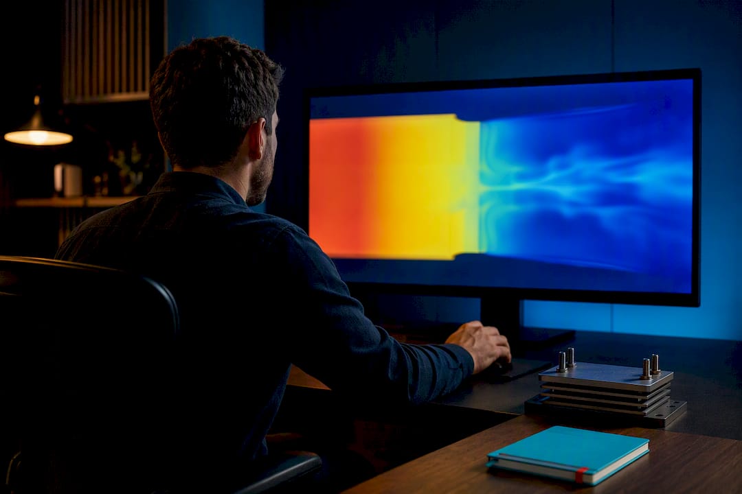
Conjugate heat transfer (CHT) is the coupled simulation of conduction in a solid and convection in an adjacent fluid, solved together so temperature and heat flux match at their shared interface. For weakly coupled problems, a partitioned solver with conservative interface enforcement works fine. For strongly coupled, multi-region problems, a monolithic or tightly coupled solver gives better stability and accuracy.
TL;DR:
Tightly coupled monolithic solvers are more stable and accurate than partitioned schemes for strongly coupled, multi-region transient conjugate heat transfer problems.
Using a Robin-Robin interface condition with appropriate relaxation factors and subcycling improves convergence and energy conservation across the solid-fluid boundary.
Mesh refinement should be applied to both solid and fluid regions simultaneously, especially in high-conductivity areas, to ensure accuracy and convergence.
Proper setup steps such as geometry cleanup, material assignment, and boundary condition selection are critical before running the solver, along with initial coarse runs for error checking.
The effectiveness of the coupling scheme depends more on interface communication strength than on mesh density alone, making the choice of solver architecture and relaxation discipline essential.
Table of Contents
What Is Conjugate Heat Transfer in CFD?
Every real thermal system has at least two things happening at once: heat moving through a solid by conduction, and heat moving through a fluid by convection (and sometimes radiation across surfaces that see each other). Conjugate heat transfer CFD solves both domains in the same simulation, exchanging temperature and heat flux across the interface instead of guessing one side and applying it as a boundary condition to the other.
Fourier’s law governs the solid side: heat flux is proportional to the temperature gradient, scaled by thermal conductivity. On the fluid side, energy moves both by conduction within the fluid and by bulk motion, which is why the fluid’s velocity field and its energy equation can’t be decoupled. At the interface itself, two physical conditions have to hold simultaneously: the temperature must be continuous (no jump between solid and fluid at the wall), and the heat flux crossing from one side must equal the heat flux arriving on the other. Get either one wrong numerically, and your junction temperatures or heat sink performance numbers will be off, sometimes badly.
Radiation adds a third mechanism that becomes non-negligible at higher temperatures or with high-emissivity surfaces facing each other. CFD models this with surface-to-surface radiation using view factors and beam tracing between patches, and skipping it in an electronics enclosure or a furnace model is a common source of error even when the conduction and convection setup is otherwise sound, as thermal analysis research on CFD-based radiation modeling points out.
Whether conduction, convection, or radiation dominates depends entirely on the geometry and materials involved:
A finned heat sink in forced air: convection and the fin’s internal conduction resistance dominate; radiation is usually a rounding error.
A motor casing in still air: conduction through the housing and natural convection at the outer skin both matter, and if the casing is dark and hot, radiation can account for a meaningful slice of total heat loss.
A furnace wall or exhaust manifold: radiation frequently rivals or exceeds convection, and ignoring it produces temperature errors that no mesh refinement will fix.
Getting a feel for which mechanism dominates before you build the model tells you where to spend meshing and solver effort, and where you can simplify without losing accuracy.
Governing Equations And Coupling Architectures
Solvers don’t all march the same energy equation forward. Some formulations track temperature directly, others solve for enthalpy, and a few use internal energy as the primary unknown. The choice matters because it changes how the solver handles variable specific heat, phase change, and compressibility. Temperature-based formulations are simplest to interpret and debug, but enthalpy formulations handle strongly temperature-dependent properties and phase-change problems more robustly. Different OpenFOAM forks reflect this split directly: several chtMultiRegionFoam variants use temperature or enthalpy as the primary variable, while foam-extend’s monolithic solver takes a different route entirely, a distinction laid out in detail in this comparative analysis of CHT coupling strategies.
That same research draws a sharp line between two coupling architectures, and understanding it is probably the single highest-leverage decision you’ll make before running a single iteration.
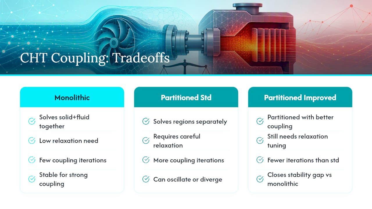
Partitioned solvers solve the solid and fluid regions as separate problems, passing boundary values back and forth each iteration or time step. They’re modular. You can swap in a different fluid solver, a different mesh, or a different turbulence model without rewriting the whole stack. The tradeoff shows up when the coupling is strong: thin, low-thermal-mass solids next to a fast-responding fluid can cause the temperature exchange to oscillate or diverge unless you’re careful with relaxation.
Monolithic solvers assemble the solid and fluid energy equations into a single system and solve them together. This costs more in terms of implementation complexity and often computational expense per iteration, but it avoids the predictor-corrector ping-pong that destabilizes partitioned schemes in tightly coupled cases.
The coupling strength trade-off: the same comparative analysis that compares foam-extend’s monolithic conjugateHeatFoam against partitioned chtMultiRegionFoam variants found monolithic approaches consistently more stable and accurate for strongly coupled, multi-region transient cases, while partitioned solvers closed much of that gap when paired with improved coupling algorithms.
In practice, most commercial and open-source CFD tools default to partitioned schemes, since it’s easier to build a general-purpose fluid solver and bolt on a solid conduction region than to write a fully coupled system. PISO and PIMPLE variants dominate the fluid side for transient cases because they handle the pressure-velocity coupling well; SIMPLE-based schemes are more common for steady-state runs where you don’t care about time accuracy, only final convergence. None of these algorithms solve the CHT interface problem by themselves. They govern how the fluid momentum and pressure fields are resolved; the temperature exchange across the solid-fluid boundary is a separate coupling loop layered on top.
If your geometry has thin, high-conductivity solids (an aluminum heat sink base, a thin metal wall separating hot and cold fluids), lean toward monolithic or a partitioned scheme with strong under-relaxation and multiple coupling iterations per time step. If the solid is thick and slow to respond thermally relative to the fluid, a standard partitioned approach with modest coupling effort will usually converge without drama.
Setting Up A CHT Model: CAD, Mesh, And Boundary Conditions
A CHT model lives or dies on setup decisions made long before the solver runs its first iteration. Vendors and open-source communities converge on roughly the same sequence, and it’s worth following in order rather than improvising:
Clean the CAD geometry first. Remove fillets, bolt holes, and cosmetic features that don’t affect the thermal path. Every unnecessary detail adds mesh cells and convergence risk for no accuracy gain.
Split the geometry into distinct fluid and solid regions. This is the step people skip when converting an existing flow-only model to CHT, and it’s non-negotiable. Each region needs its own material assignment and its own mesh treatment.
Decide which thin solids can be simplified. A 0.2mm coating or a thin gasket often doesn’t need its own meshed region; a thermal contact resistance or a thin-wall boundary condition captures the same physics for far less mesh cost.
Mesh the fluid region with wall-normal resolution matched to your turbulence model. Target a y+ near 1 for models that resolve the boundary layer directly, or use wall functions with a coarser first cell if you’re using a high-Reynolds turbulence model. Add inflation layers (5 to 15 layers is typical) to capture the steep temperature and velocity gradients near walls, since this is exactly where convective heat transfer coefficients are computed.
Choose conformal or non-conformal meshing at the interface. Conformal meshes (matching node locations across the fluid-solid boundary) give the cleanest flux transfer but constrain your meshing strategy on both sides. Non-conformal interfaces (using interpolation like GGI or arbitrary mesh interface methods) give you meshing freedom at the cost of some interpolation error, which matters more as the temperature gradient at the interface gets steeper.
Assign temperature-dependent material properties wherever the operating range justifies it. Thermal conductivity and specific heat can vary meaningfully across a wide temperature swing, and treating them as constants when they’re not is one of the most common accuracy failures in CHT work.
Set boundary conditions deliberately, not by default. Decide whether you know the heat flux or the temperature at each external boundary. Prescribing the wrong one, or prescribing both where only one is physically known, is a frequent modeling error. Inlet turbulence intensity and thermal boundary layer thickness also need real values, not solver defaults, especially in developing flow.
This sequence mirrors the CHT setup workflow that SimScale documents as CAD cleanup, region operations, material assignment, boundary conditions, solver selection, and result controls, and it’s a good checklist to keep next to your model tree.
Pro Tip: Build a coarse, fast-running version of your full CHT model before you invest in the fine mesh. Running the coarse version end-to-end first catches boundary condition mistakes, sign errors on heat flux, and region-assignment bugs in minutes instead of after an eight-hour fine-mesh run fails to converge.
CFD earns its keep in exactly this kind of problem because it resolves the flow pattern, the turbulence structure, and the resulting temperature field together, something analytical heat transfer methods simply can’t do once the geometry gets complicated.
How Do You Enforce The Interface Condition Numerically?
The physics says temperature and heat flux must match at the solid-fluid boundary. The numerics say you have to pick a specific way to enforce that match, and the choice affects both how fast your simulation converges and how physically accurate the result is.
Dirichlet-Dirichlet: both sides get a prescribed temperature. Simple to implement, but it doesn’t naturally conserve heat flux across the interface unless you iterate carefully.
Neumann-Neumann: both sides exchange heat flux instead of temperature. Conserves energy by construction, but can be slow to converge when thermal diffusivities on either side differ substantially.
Dirichlet-Robin: one side gets a fixed temperature, the other gets a mixed condition combining temperature and flux. A common middle ground.
Robin-Robin: both sides use a weighted combination of temperature and flux, with the weighting tuned to the relative thermal diffusivities of the two regions. This is generally the most robust option for problems with a large mismatch in thermal properties across the interface, a point the research on CHT coupling strategies makes in detail when comparing implementation classes for convergence and conservation.
Relaxation factors on the coupling loop matter almost as much as which scheme you pick. Starting too aggressively (under-relaxation factors above 0.7 for temperature exchange in a tightly coupled case) is the fastest way to watch a residual plot start oscillating and never settle. A safer starting point for a new CHT case is somewhere in the 0.3 to 0.5 range on the interface temperature update, tightening toward 0.7 or higher only once you’ve confirmed the case is converging cleanly at the conservative setting.
Time-stepping introduces its own wrinkle when fluid and solid thermal time scales are far apart, which happens often: a thin fluid boundary layer responds in milliseconds while a thick metal casing takes minutes to heat up. Subcycling the fluid solver several times per solid time step, or using a semi-analytical coupling scheme for the slow side, keeps you from either wasting compute resolving the fluid at the solid’s glacial pace or under-resolving fast fluid transients. This is a genuinely advanced tweak, not a default setting, and it’s worth reaching for only once a standard time step has proven too coarse or too expensive.
Keeping A CHT Simulation Stable And Accurate
Divergence in CHT models rarely comes from one dramatic mistake. It usually comes from a stack of small numerical choices that individually look fine and collectively push the solver past what it can handle.
Residual tolerances are the first thing to set deliberately rather than accept by default. For steady-state runs, driving continuity and energy residuals down three to four orders of magnitude from their starting value is a reasonable target before trusting the result; transient runs need tighter inner-iteration convergence per time step, since errors compound across steps in a way steady solutions never see.
Time step selection should respect two separate constraints, not just one. The Courant-Friedrichs-Lewy (CFL) condition bounds the step size based on flow velocity and cell size. A separate thermal diffusion stability criterion bounds it based on how fast heat spreads through the solid mesh, and in problems with thin, highly conductive solids, this second constraint is often the tighter one. Checking only CFL and ignoring the thermal diffusion limit is a common reason CHT transients diverge even when the flow field looks stable.
Track the interface heat flux imbalance between regions every iteration, not just the global residuals.
Watch for oscillating interface temperature between coupling iterations. Growing oscillation almost always means your relaxation factor is too aggressive for the coupling strength you’re dealing with.
Confirm total energy in equals total energy out (plus storage, for transient runs) as a conservation sanity check before trusting any local temperature number.
Mesh convergence testing in CHT means refining both regions together, not just the fluid mesh. Refining only the fluid side while leaving a coarse solid mesh in a strongly conducting part will plateau your accuracy well before the fluid-side residuals suggest you’re done. Structured guidance on grid refinement, adaptive meshing, and the computational tradeoffs involved is covered well in classic CFD numerical methods references, including the discretization and parallel-processing strategies discussed in Computational Fluid Dynamics.
A useful diagnostic once your model runs cleanly: rerun it with the interface coupling scheme switched (Dirichlet-Robin to Robin-Robin, for instance) and confirm the converged temperature field barely moves. If it shifts meaningfully, your original scheme wasn’t actually converged. It just looked stable.
Proving Your CHT Model Is Right, Not Just Stable
A model that converges isn’t automatically a model you can trust. Verification and validation are two separate questions, and skipping either one is how bad numbers make it into a design review.
Run the conservation check first. Confirm energy entering the domain equals energy leaving it, plus any storage term you’d expect in a transient case. A mismatch here means a setup error, not a mesh problem.
Check interface flux continuity directly. Heat flux computed on the solid side of the interface should match the flux computed on the fluid side to within a small tolerance. Large mismatches usually trace back to non-conformal interface interpolation error or an under-resolved boundary layer.
Run a proper mesh convergence study across both regions. Refine solid and fluid meshes together in at least two or three steps, and confirm your key output (junction temperature, exit fluid temperature, heat sink base temperature) stops changing meaningfully between the two finest levels.
Compare against an experimental or published benchmark case where one exists. Classic CHT benchmarks like a heated cylinder in cross-flow or a finned heat sink with measured junction temperatures give you a sanity check that pure mesh convergence can’t provide, since a model can converge to the wrong physics just as easily as the right one.
Report uncertainty honestly. State the percentage difference between your finest two mesh levels, not just the final number, and note where boundary condition assumptions (fixed heat flux versus a real convective boundary, for instance) could shift the result if they’re wrong.
Where CHT Simulation Shows Up In Real Engineering Work
Electronics cooling is probably the most common CHT application engineers run into: predicting junction-to-ambient temperature rise across a heat sink under forced convection requires solving the fin’s internal conduction and the airflow’s convective coefficient together, since neither one alone tells you the junction temperature. Heat sink CFD work lives almost entirely in this territory.
Heat exchangers and rotating machinery add another layer: multiple fluid regions, sometimes a rotating solid region relative to a stationary casing, and moving-wall boundary conditions that have to stay synchronized with the mesh motion.
The two mistakes that show up most often: treating conductivity and specific heat as constant across a wide operating temperature range, and letting the interface mesh mismatch between conformal regions get too coarse relative to the temperature gradient there. Both are cheap to avoid and expensive to diagnose after the fact.
Where To Go Deeper On CHT Modeling
Joel has written extended, step-by-step coverage of conjugate heat transfer workflows, including a full walkthrough of CHT simulation for engineers and a companion piece mapping governing equations to solver setup for readers who want the math connected directly to solver options. Jewlz Technologies also builds physics-based simulation tools, including CFD simulation software, for engineers who want to move from theory straight into a working model.
The Bottom Line On CHT Solver Choice
Coupling strength decides your solver, not habit or software defaults. Before running anything, check:
Region split and mesh quality at the interface
Correct boundary condition type (flux or temperature) on every surface
Relaxation factors matched to coupling strength
Mesh convergence across both regions
A benchmark or conservation check confirming the result is physically real
Why Most CHT Guides Get The Coupling Question Backward
Most advice on this topic treats “partitioned versus monolithic” as a software feature comparison, when it’s actually a physics question in disguise. The right question isn’t which solver architecture you have access to. It’s how tightly your solid and fluid regions actually talk to each other. A thick aluminum block next to slow-moving air can get away with a loose partitioned scheme and sloppy relaxation factors. A 1mm copper fin next to fast-moving forced air cannot, and no amount of mesh refinement will rescue a coupling scheme that’s fundamentally too weak for that interaction.
The overrated piece of conventional wisdom is mesh density. Engineers pour hours into refining the fluid mesh while running a coarse, constant-property solid region, then wonder why their junction temperature won’t converge. The underrated piece is relaxation factor discipline on the interface itself. Get that wrong and a beautiful mesh just converges slowly to the wrong answer.
Start every new CHT case by classifying the coupling strength honestly, then choose the solver architecture and interface scheme to match. Everything else, mesh resolution, turbulence model, radiation treatment, is secondary to getting that first decision right.
— Joel
Get Hands-On With Thermal Simulation Tools
Building a CHT model by hand in a general-purpose CFD package takes real setup time before you see a single useful number. Jewlztech built its thermal analysis toolkit specifically to shorten that gap: variable material properties, a built-in property database, and support for conduction, convection, and radiation modes in one downloadable Excel-based tool, so you’re not rebuilding property tables and boundary condition logic from scratch on every project.

It suits engineers and students who need reliable thermal numbers without standing up a full CFD environment for every quick check, and it pairs naturally with the CFD simulation software for readers who need the full coupled solve described in this guide. If you’re starting your first CHT model this week, open the thermal analysis toolkit and run your boundary conditions through it before you commit to a mesh.
Sources
Recommended
Comments