
Conjugate Heat Transfer: Simulation Guide for Engineers

Updated: Sep 16
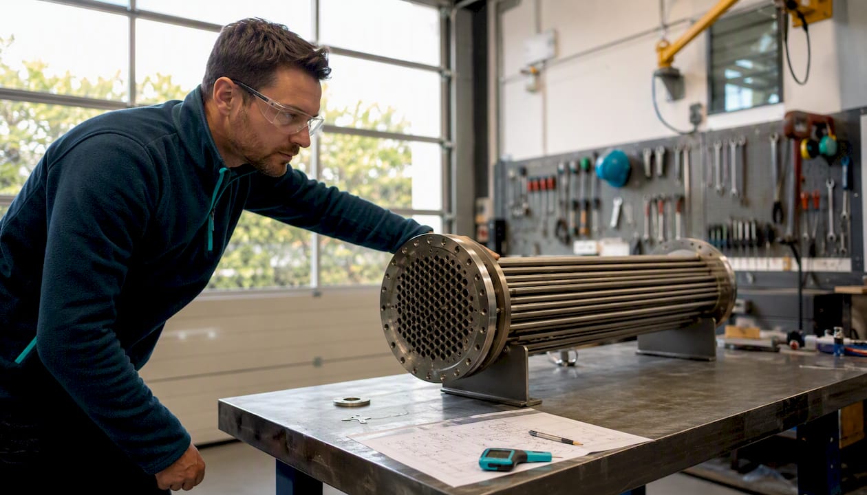
Conjugate heat transfer (CHT) is the simultaneous solution of thermal fields in both a solid and an adjacent fluid, with temperature and heat flux matched continuously at their shared interface. No assumed convection coefficient. No empirical shortcut. The physics in both domains are solved together, which is why CHT is the right modeling choice when the solid and fluid are tightly thermally coupled, when boundary layer behavior drives the temperature distribution in the wall, or when you are dealing with multimode problems like battery packs, electronics cooling, or turbine blade aero-thermal analysis. The trade-off is real: a CHT simulation typically costs one to two orders of magnitude more compute time than a simple h-based boundary condition model, so the decision to use it should be deliberate.
Table of Contents
What conjugate heat transfer actually is (and why h-based models fall short)
When CHT is necessary and when a simpler model is good enough
Running a validation example: grid convergence and energy balance checks
Why CHT changes engineering decisions more than people expect
The Thermalysis Toolkit handles the CHT workflow you just read about
What conjugate heat transfer actually is (and why h-based models fall short)
Conjugate convective heat transfer was formalized in the mid-20th century as a way to replace the empirical convection coefficient with a mathematically consistent interface condition. Instead of prescribing h at the wall, you solve the energy equation in the solid and the fluid separately, then enforce two conditions at the interface: temperature continuity and heat flux continuity.
The interface energy balance is the load-bearing constraint of the whole approach:
Temperature on both sides of the interface must match, and the conductive flux leaving the solid must equal the convective flux entering the fluid. That single condition is what removes the need for an assumed h and lets you compute local heat transfer coefficients from first principles, which matters enormously for compact electronics and tightly coupled systems where h varies spatially by factors of two or more.
The practical difference between CHT and an h-based model comes down to what you know before you start:
Criterion | CHT (physics-based) | Empirical h-method |
Input required | Geometry, material properties, flow BCs | Prescribed h or Nusselt correlation |
Accuracy at interface | High; local h computed from solution | Depends on correlation validity |
Handles complex geometry | Yes | Only if a correlation exists |
Computational cost | High | Low |
Best for | Tight coupling, novel geometries, design optimization | Well-characterized flows, early scoping |
The h-method is not wrong. For a straight pipe with fully developed turbulent flow, a Dittus-Boelter correlation is fast and accurate. CHT earns its cost when the geometry is complex, the coupling is strong, or you need local temperature distributions rather than bulk averages.
Which heat transfer modes show up in a CHT problem
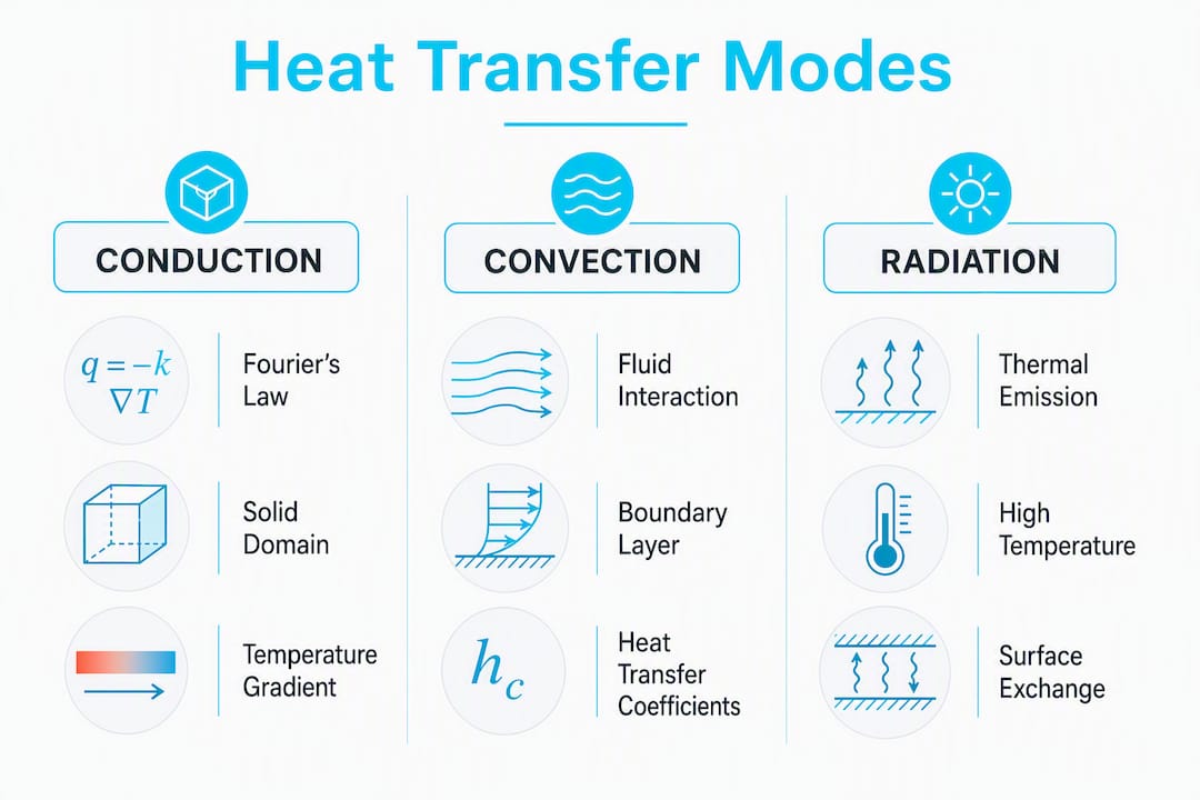
Most CHT problems involve at least two modes, and real-world cases often involve all three.
Conduction governs the solid domain. Heat moves through the material according to Fourier’s law, and the temperature gradient in the solid directly sets the flux delivered to the interface. Material thermal conductivity, density, and specific heat all matter, and they are often temperature-dependent in the ranges engineers care about.
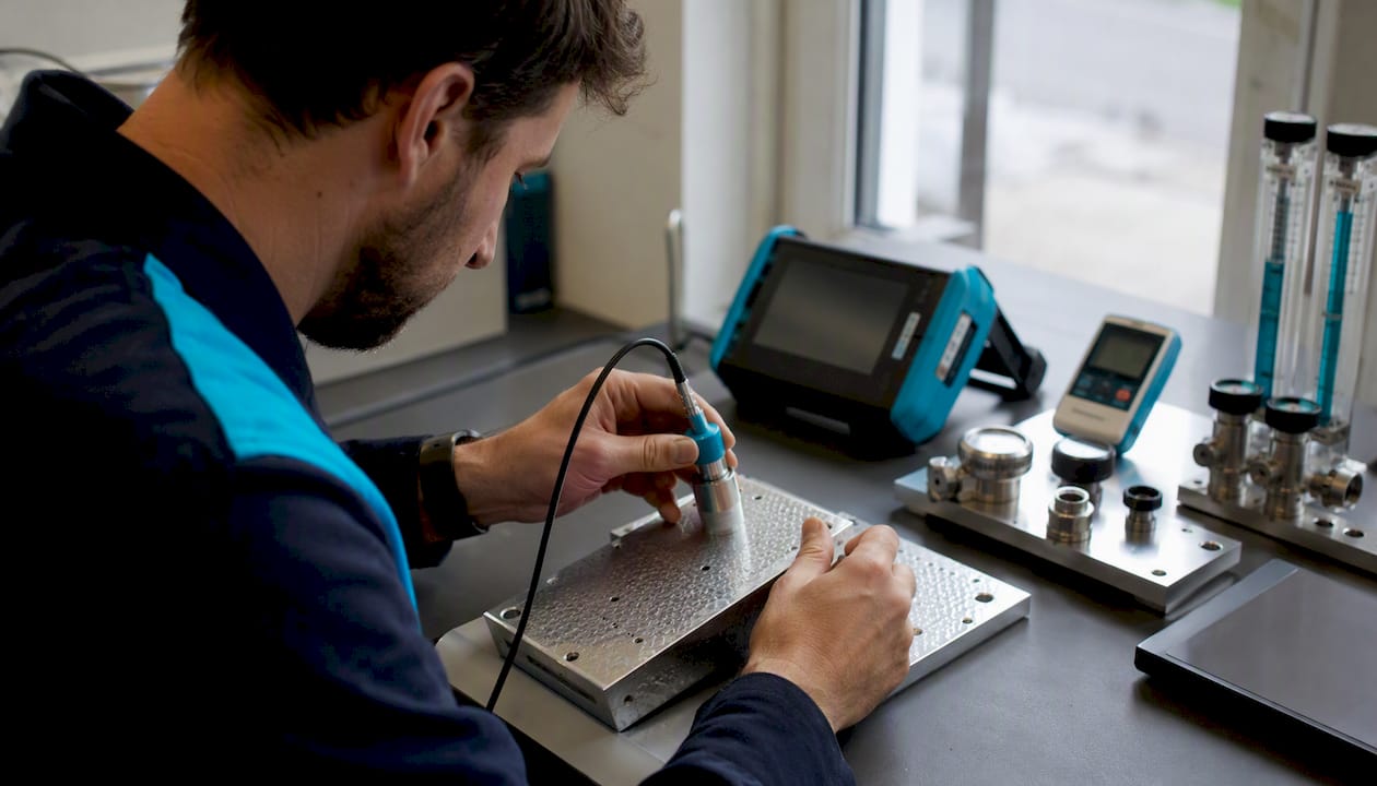
Convection governs the fluid domain. The boundary layer adjacent to the solid wall is where the thermal coupling happens. In laminar flow the boundary layer is smooth and relatively easy to resolve. In turbulent flow, the near-wall region requires careful treatment, and the choice of wall model has a direct effect on the predicted interface flux.
Radiation is the mode most commonly dropped without justification. For many electronics cooling problems at moderate temperatures, that is defensible. For battery modules, turbine components, and any geometry with closely spaced surfaces at elevated temperatures, neglecting radiation leads to wrong answers. Research on multi-mode heat transfer in Li-ion battery packs shows that both radiation and natural convection meaningfully affect thermal runaway propagation, and that the interstitial material conductivity interacts with those modes in non-obvious ways.
Mass-coupled heat transfer appears when species transport or phase change is present, such as in evaporative cooling or electrochemical systems. It adds another coupling term to the interface balance and is beyond the scope of most introductory CHT setups, but worth flagging when the physics demand it.
Pro Tip: A practical rule for radiation inclusion: if any surface in your model exceeds a high temperature threshold, or if surface emissivities are high and surfaces face each other within a small gap, include radiation. Below those thresholds in a forced-convection-dominated problem, the radiation contribution is usually small enough to ignore. When in doubt, run a quick sensitivity case with and without radiation before committing to the full model.
For a worked look at how conduction, convection, and radiation interact in practical setups, the Jewlztech blog has teaching-oriented examples that map well to the multimode coupling described here.
The governing equations behind CHT
The solid domain is governed by the transient heat conduction equation:
where ρ_s is solid density (kg/m³), c_s is specific heat (J/kg·K), k_s is thermal conductivity (W/m·K), and Q_s is any volumetric heat source (W/m³). In steady state, the left side drops to zero.
The fluid domain requires the energy equation coupled to the Navier-Stokes system. The energy equation in the fluid takes the form:
where u is the velocity field (m/s) and Φ captures viscous dissipation, which is relevant at high speeds or high-viscosity flows. The continuity and momentum equations close the system.
At the interface, two conditions must hold simultaneously:
T_solid = T_fluid (temperature continuity)
(n · k_s ∇T)_solid = (n · k_f ∇T)_fluid (heat flux continuity)
Boundary conditions on the outer surfaces follow the usual categories. A Dirichlet condition fixes temperature (T = T_wall). A Neumann condition prescribes flux (n · k∇T = q_specified, or zero for an insulated surface). A convective or Robin condition applies an external h and ambient temperature when the far-field is not resolved in the model.
Heat transfer analysis at the level required for CHT always demands temperature-dependent material properties. Conductivity, specific heat, and emissivity all vary with temperature, and using constant values across a wide operating range introduces systematic error that no amount of mesh refinement will fix.
How CHT problems are solved numerically
Two broad strategies exist, and the choice between them shapes everything from solver stability to runtime.
Monolithic (fully coupled) solvers assemble the solid and fluid energy equations into a single system and solve them simultaneously. The interface conditions are enforced implicitly within the matrix. This approach is unconditionally consistent at the interface and handles fast transients well, but the system matrix is larger and more expensive to invert. It is the preferred choice for problems where the thermal time scales in the solid and fluid are similar.

Partitioned (loosely coupled or staggered) solvers solve the fluid and solid domains sequentially, passing boundary data between them at each time step or iteration. The Fuego solver from Sandia National Laboratories implements a temperature-forward, flux-back scheme: the fluid is solved using the solid surface temperature as a Dirichlet boundary condition, then the resulting fluid flux is applied to the solid as a Neumann condition. This is computationally cheaper per step, but it introduces temporal splitting errors and can miss energy balance within a time step for fast transients. Fuego’s documentation explicitly warns about interpolation errors when fluid and solid meshes do not conform at the interface.
For transient problems with strong thermal gradients, loosely coupled algorithms improve efficiency but can fail to converge the interface energy balance within a timestep. The fix is iterative coupling: run multiple fluid-solid exchange iterations per time step until the interface flux residual drops below a tolerance. This adds cost but restores accuracy.
Turbulence modeling adds another layer of decision-making. When the boundary layer is fully resolved (y⁺ ≈ 1), the near-wall temperature gradient is computed directly and the interface flux is accurate. When wall functions are used (y⁺ in the range of 30–300), the first fluid node sits away from the wall and the heat flux is reconstructed using a law-of-the-wall. Wall functions are faster but require validated correlations and careful scrutiny of near-wall flux predictions.
Pro Tip: For a first CHT run, start with a steady-state monolithic solve and a coarse mesh to verify that the interface conditions are being applied correctly and that the energy balance closes. Only then refine the mesh and switch to transient if the physics require it. Debugging a transient, loosely coupled, turbulent CHT case from scratch is a reliable way to lose a week.
A practical setup checklist for your first CHT simulation
Follow this sequence when building a CHT model. Skipping steps, especially geometry cleanup and interface definition, causes problems that are hard to diagnose later.
Clean the geometry. Remove small features below the mesh resolution target. Shared surfaces between solid and fluid domains must be geometrically coincident, not just visually close. Gaps or overlaps at the interface break the coupling.
Define material properties with temperature dependence. Pull conductivity, specific heat, and density as functions of temperature for every solid material. For fluids, include viscosity and thermal conductivity variation. Modern heat transfer analysis treats temperature-dependent properties as standard, not optional.
Set interface and contact definitions explicitly. In most solvers, the CHT interface must be declared as a coupled boundary, not a wall with a fixed temperature. Verify that the solver is enforcing both temperature and flux continuity, not just one.
Build the mesh with the interface in mind. Refine near the solid-fluid interface. For wall-resolved turbulent flow, target y⁺ ≈ 1 at the first fluid cell. For wall-modeled approaches, target y⁺ in the 30–300 range and use validated wall functions.
Wall treatment | Target y⁺ | Mesh cost | Accuracy at interface |
Wall-resolved (low-Re) | ≈ 1 | High | High |
Wall-modeled (wall functions) | 30–300 | Moderate | Moderate; correlation-dependent |
Apply boundary and initial conditions. Set inlet velocity/temperature, outlet pressure, and external surface conditions. For transient cases, initialize with a physically reasonable temperature field, not zero everywhere.
Choose solver controls. For steady CHT, use implicit solvers with under-relaxation. For transient CHT, set the time step so the Courant number stays below 1 in the fluid near the interface. Enable coupling iterations if using a partitioned solver.
Run a mesh convergence study before trusting any result. Refine the mesh by a factor of 1.5–2 in each direction near the interface and compare interface temperatures and fluxes. Mesh-convergence studies are among the most commonly skipped steps in heat transfer analysis and among the most consequential.
Postprocess the interface energy balance. Integrate the heat flux over the interface on both the solid and fluid sides. The two values should match to within your solver’s convergence tolerance. A mismatch signals a coupling error, not a physics insight.
Pro Tip: For transient CHT, run a short time-step sensitivity study early: halve the time step and check whether the interface temperature history changes. If it does, your original step was too large. This takes an hour and can save days of rerunning a long simulation.
Where CHT is used in engineering practice
CHT appears wherever the solid temperature distribution and the fluid flow are mutually dependent. These are the domains where it shows up most often:
Electronics and PCB cooling. Component junction temperatures depend on the local airflow pattern, which depends on the board layout and heat spreader geometry. An h-based model cannot capture the spatial variation in convective intensity across a populated board. CHT resolves local hotspots and lets you evaluate design changes before fabrication. A useful postprocessing output is a combined temperature contour and velocity streamline plot showing where the boundary layer thickens and where heat accumulates.
Heat exchangers. Shell-and-tube and plate heat exchangers involve thin walls separating hot and cold streams. The wall conduction resistance is part of the thermal circuit, and CHT captures it directly. For heat exchange problems with fouling or variable wall thickness, CHT is the only way to get accurate local effectiveness predictions.
Li-ion battery packs. Thermal runaway propagation depends on conduction through cell casings, convection in the cooling channel, and radiation between closely spaced cells. Research confirms that both radiation and natural convection affect runaway behavior, and that interstitial conductivity has a non-monotonic effect on propagation. Simplified h-based models miss these interactions entirely.
Turbine blades and aero-thermal components. Film cooling, internal cooling channels, and the hot gas path all interact thermally through the blade wall. CHT is standard practice in turbine aerothermal design, and high-speed external flow CHT at transonic and supersonic conditions adds compressibility effects to the coupling.
Automotive and aerospace thermal management. Exhaust manifolds, brake rotors, and heat shields all involve solid components bathed in high-temperature flows where the wall temperature distribution drives material stress calculations downstream.
For a broader look at heat transfer applications across these domains, the Jewlztech engineering reference covers the modeling choices that map to each use case.
When CHT is necessary and when a simpler model is good enough
CHT is not always the right tool. Knowing when to step back saves significant compute time.
Use CHT when:
The solid and fluid thermal time scales are comparable (neither dominates).
Local temperature distributions in the solid matter for stress, material selection, or safety analysis.
The geometry is complex enough that no validated correlation exists for h.
You need to evaluate design changes that alter the flow pattern and the wall temperature simultaneously.
Radiation between surfaces is significant (see the rule of thumb in the physical modes section).
An empirical h-method is acceptable when:
The flow regime and geometry match a well-validated Nusselt correlation.
You need a fast scoping estimate and the interface temperature is not the primary output.
The solid thermal resistance is negligible compared to the convective resistance (thin, highly conductive walls).
You are doing parametric sweeps where relative trends matter more than absolute accuracy.
Computational cost planning. A small CHT problem (a single chip on a board, a short pipe section, a few thousand cells per domain) typically runs in minutes to tens of minutes on a modern workstation. A medium problem (a full PCB, a multi-pass heat exchanger, a battery module with a dozen cells) runs in hours. A large, high-fidelity transient CHT case (a full turbine stage, a battery pack with thermal runaway, a data center row) can run for days even on a cluster. Budget accordingly, and always run the coarse steady-state case first.
Practical limitations worth flagging: mesh resolution near the interface drives memory requirements up fast, especially for wall-resolved turbulent cases. Solver stability in partitioned schemes requires careful time-step control. And every CHT result needs experimental or benchmark validation before it informs a design decision.
Software and learning resources for CHT practice
The CHT software ecosystem spans open-source research codes, academic multiphysics frameworks, and commercial packages. The right choice depends on your access, budget, and the complexity of the problem.
Open-source and research codes include solvers with explicit partitioned coupling (temperature-forward, flux-back schemes like the one documented in Fuego) and fully coupled multiphysics frameworks. The MOOSE framework from Idaho National Laboratory implements CHT through interface kernels that enforce the coupled temperature-flux condition directly, and its documentation includes worked benchmark cases. OpenFOAM has a chtMultiRegionFoam solver that handles multi-region CHT with conjugate interfaces and is widely used in academic research.
Commercial multiphysics packages with monolithic solvers include COMSOL Multiphysics, which has a dedicated Heat Transfer Module with built-in CHT interface conditions, temperature-dependent material libraries, and tutorial cases covering electronics cooling, heat exchangers, and battery thermal management. SimScale offers browser-based CHT simulation with guided workflows and a library of example cases, which makes it accessible for students and early-career engineers who want to run CHT problems without a local HPC setup.
Where to find validation tutorials. The most reliable tutorials are those that include a comparison against experimental data or an analytical benchmark. COMSOL’s application gallery and SimScale’s public project library both tag cases with validation status. The ASEE finite-difference multi-mode heat transfer project is a well-structured academic example that covers conduction, convection, and radiation with both steady-state and transient versions and comparison to analytical solutions.
For solver category comparisons without vendor lock-in, the Jewlztech post on simulation software alternatives covers feature categories and trade-offs that map directly to the CHT workflow choices described here.
Running a validation example: grid convergence and energy balance checks
A CHT result you cannot verify is a result you cannot use. This is the sequence every engineer should run before reporting or acting on a CHT simulation.
Define the case clearly. Choose a geometry with a known benchmark or experimental result: a heated channel with a solid wall, a fin array, or a simple electronics package. Document the geometry, material properties, boundary conditions, and solver settings before running anything.
Run three mesh levels. Start with a coarse mesh, then refine by a factor of 1.5–2 near the interface for the medium and fine levels. Record the interface temperature, the total heat flux through the interface, and the maximum solid temperature at each level.
Check grid convergence. If the interface temperature changes by less than 1–2% between the medium and fine meshes, the solution is grid-independent for that quantity. If it is still changing, refine further or investigate whether the mesh is resolving the boundary layer correctly.
Verify the interface energy balance. Integrate heat flux over the interface on both sides. The solid-side integral and the fluid-side integral should match. A mismatch larger than your solver’s stated convergence tolerance indicates a coupling error.
Monitor residuals and probe temperatures. Plot residuals for energy, momentum, and continuity over iterations or time steps. Residuals that plateau without converging often signal a time-step or coupling-iteration problem. Place temperature probes at the interface and at representative interior points and confirm they reach steady values (or physically meaningful transient behavior).
Run a sensitivity study on turbulent Prandtl number. For turbulent CHT, the turbulent Prandtl number (Pr_t, typically 0.85–0.9 for air) affects the predicted wall heat flux. Vary it by ±10% and check the sensitivity of the interface temperature. If the result is highly sensitive, your wall treatment needs scrutiny.
Document everything for reproducibility. Record mesh counts, y⁺ statistics, solver settings, convergence criteria, and the grid-convergence table. A result that cannot be reproduced from documentation is not a result.
Key Takeaways
Conjugate heat transfer requires simultaneous solution of solid and fluid thermal fields with enforced interface energy continuity, making it the right choice when coupling is tight, geometry is complex, or local temperature distributions drive design decisions.
Point | Details |
Interface condition is the core | Temperature and heat flux must both be continuous at the solid-fluid boundary; this replaces the assumed h. |
Monolithic vs partitioned trade-off | Monolithic solvers are more accurate for fast transients; partitioned schemes are cheaper but need iterative coupling for high-gradient cases. |
Mesh convergence is non-negotiable | Run at least three mesh levels and verify interface flux convergence before trusting any CHT result. |
Radiation matters in packed systems | For battery modules and high-temperature components, neglecting radiation leads to wrong propagation and hotspot predictions. |
Jewlztech Thermalysis Toolkit | Supports temperature-dependent properties, multiphysics coupling, and built-in validation examples for CHT workflows. |
Why CHT changes engineering decisions more than people expect
The conventional wisdom treats CHT as a premium modeling choice you reach for when accuracy demands it. That framing undersells what actually happens when you switch from an h-based model to a fully coupled solution.
The real value is not just better numbers. It is that CHT surfaces spatial structure in the temperature field that empirical models average away. A uniform h assumption tells you the mean wall temperature. CHT tells you where the hotspot is, how sharp it is, and how it moves when you change the flow rate or the geometry. That difference has driven real design rework: cooling channels repositioned, fin pitches changed, thermal interface materials selected based on local conductivity requirements rather than bulk estimates.
The practical advice most guides skip: do not wait for a full CHT simulation to inform every decision. Use h-based scoping to narrow the design space first, then commit CHT resources to the two or three configurations that survive that screen. The engineers who get the most out of CHT are not the ones who run it on everything. They are the ones who know exactly which design question requires the spatial resolution that only a coupled solution can provide.
For decisions about active versus passive cooling strategies, the thermal modeling outcomes from CHT feed directly into the design choice. Running CHT without a plan for how the result changes the decision is expensive and often unnecessary.
The Thermalysis Toolkit handles the CHT workflow you just read about
Running a CHT simulation from scratch means managing temperature-dependent material properties, interface coupling definitions, mesh strategy, and validation checks simultaneously. The Thermalysis Toolkit from Jewlztech is built around exactly that workflow: it supports variable material properties across a wide temperature range, covers conduction, convection, and radiation in a single environment, and includes a built-in property database so you are not hunting for conductivity curves mid-setup.

The Thermalysis Toolkit is a web-based engineering application, giving engineers direct browser access to thermal analysis tools without requiring a specialized desktop installation or license server. Users can access available features immediately, while the full toolkit provides expanded multiphysics analysis capabilities and engineering validation tools. If you are working through the simulation checklist in this guide and want a structured environment to apply these methods, the Thermalysis Toolkit is a practical place to start. Visit the product page to explore the available features and applications.
Useful sources
These references cover the theory, numerical methods, and benchmark cases that underpin the guidance in this article. Prioritize sources that include experimental or analytical validation alongside the simulation results.
MOOSE Framework: ConjugateHeatTransfer Interface Kernel — Documents the interface kernel implementation enforcing coupled temperature-flux conditions; includes worked benchmark cases useful for verifying your own setup.
Fuego User Manual: Conjugate Heat Transfer (Sandia National Laboratories) — Detailed treatment of partitioned coupling, the temperature-forward flux-back scheme, mesh conformance requirements, and wall function treatment for turbulent CHT.
Conjugate Convective Heat Transfer (Wikipedia) — Concise historical and formulation overview; useful for understanding the original Perelman (1961) and Sparrow (1968) formulations that established the interface matching conditions.
Multi-Mode Heat Transfer Simulations of Thermal Runaway in Li-Ion Cells (IOPscience) — Research paper with experimental validation of multimode CHT in battery packs; directly relevant for anyone modeling thermal runaway or battery thermal management.
Conjugate Heat Transfer in High-Speed External Flows (AIAA Journal) — Covers CHT at transonic and supersonic conditions with compressibility effects; benchmark cases included.
Design of a Multi-Mode Finite Difference Heat Transfer Project (ASEE) — Academic project covering conduction, convection, and radiation in a single finite-difference framework with steady-state and transient versions; includes comparison to analytical solutions, making it a strong starting point for students.
Recommended
Comments