
Bi <0.1? Use Lumped Capacitance, Biot Number Criteria for Engineers

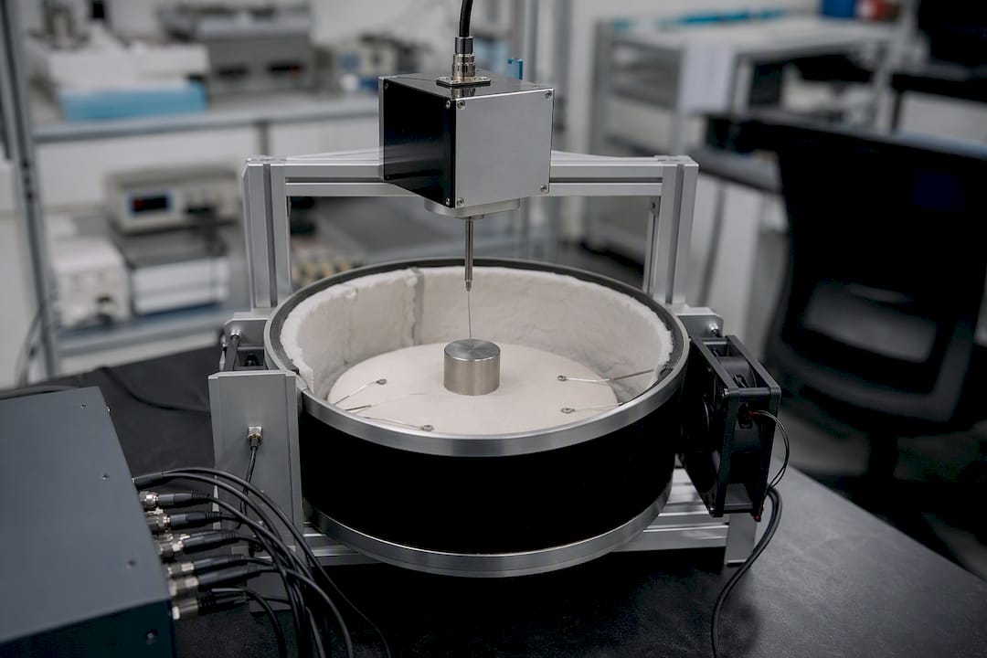
The Biot number, Bi = h·Lc/k, tells you whether a solid heats or cools uniformly enough to skip solving a full conduction equation. If Bi comes out below 0.1, the lumped-capacitance method applies, treating the whole object as one temperature with roughly less than 5% error. Above that, internal temperature gradients are significant and require more complex analysis methods, with the magnitude of Bi guiding the choice.
TL;DR:
A Biot number below 0.1 indicates the lumped-capacitance model is accurate, but higher values require more complex analysis to account for internal temperature gradients.
The characteristic length is usually the volume divided by exposed surface area, with shape-specific shortcuts for common geometries like spheres and cylinders.
Internal conduction resistance always uses the solid’s thermal conductivity, not the fluid’s, to correctly assess heat transfer and gradient significance.
As convective heat transfer coefficient increases, the Biot number rises, making the lumped model less reliable and necessitating numerical solutions for large or complex Bi values.
Regular checks of the Biot number are essential during design iterations, especially when geometries or convection conditions change, to determine the appropriate thermal analysis method.
Table of Contents
What Is the Biot Number Formula and Why Does It Work?
Bi comes from comparing two resistances to heat flow. Internal conduction resistance scales with Lc/k, where k is the solid’s thermal conductivity. Surface convection resistance scales with 1/h, where h is the convective heat transfer coefficient. Divide one by the other and the units cancel: (Lc/k) / (1/h) = h·Lc/k. That is the whole derivation, and it’s why Thermopedia and most heat transfer textbooks frame Bi as a resistance ratio rather than a formula to memorize.
The payoff of that framing: when Bi is small, conduction resistance is negligible compared to convection resistance. Heat moves through the solid so much faster than it leaves the surface that the interior stays essentially uniform in temperature. When Bi is large, the opposite happens. The surface reaches the fluid temperature almost immediately while the core lags behind, sometimes by a wide margin.
One detail trips up a lot of students here. The k in Bi is always the solid’s conductivity, not the fluid’s. That distinction matters more than it sounds like it should, because a nearly identical-looking dimensionless group, the Nusselt number, uses fluid conductivity instead. Mixing the two up produces a number that looks reasonable but means nothing physically.
How Do You Choose the Characteristic Length Lc?
The standard convention, used across ScienceDirect’s treatment of transient conduction and most modern textbooks, is Lc = V / As, the body’s volume divided by its exposed surface area. This convention generalizes cleanly across shapes and matches the way lumped-capacitance solutions are actually derived, so it’s the default unless you’re working from a chart or reference that specifies otherwise.
For common shapes, that ratio reduces to simple rules:
Sphere: Lc = R/3, where R is the radius.
Long cylinder: Lc = R/2, using the radius, when convection acts on the curved surface only.
Slab cooled or heated from both faces: Lc = half the thickness.
Slab exposed on one face only (insulated on the other): Lc equals the full thickness.
That last point catches people off guard. If one side of a plate is insulated or attached to another material, only the exposed surface counts toward As. Using the total surface area of an object that’s only losing heat from part of it will understate Bi and can lead you to trust a lumped model that doesn’t actually apply.
A quick checklist before you commit to a value of Lc:
Confirm which surfaces are actually exposed to the convective fluid.
Match your Lc convention to whatever solution method you’ll use next (some Heisler charts define characteristic length differently, often as the full radius or half-thickness rather than V/As).
Recompute Bi if geometry or exposure changes partway through a design.
When Does the Lumped-Capacitance Method Apply?
The widely cited criterion is straightforward: Bi < 0.1 means lumped capacitance is valid, with error in the predicted temperature history staying under roughly 5% compared to the exact solution. Below that threshold, treating the object as a single thermal mass with one uniform temperature can be a reasonable simplification.
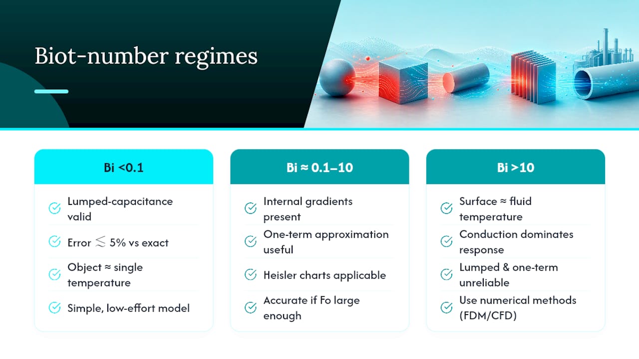
Between Bi ≈ 0.1 and Bi ≈ 10, the situation gets more interesting. Internal gradients exist but aren’t extreme enough to require a full numerical solution. This is exactly the range where the one-term approximation and Heisler charts earn their keep. These tools give you the center and surface temperature histories for simple geometries (spheres, infinite cylinders, infinite slabs) without solving a partial differential equation by hand, and they remain accurate as long as the Fourier number is large enough for the series solution to be dominated by its first term.
Once Bi climbs past roughly 10, the surface behaves almost like it’s instantly matching the fluid temperature, and the object’s own conduction dominates the response entirely. At this point neither the lumped model nor the simple one-term chart is reliable. Complex geometry, temperature-dependent material properties, or genuinely large Bi all point toward a numerical solution, whether that’s a finite-difference conduction code or a full CFD simulation that couples the solid and fluid domains together.
How Do You Calculate Bi and Decide on a Method?
Here’s a repeatable process you can apply to almost any transient heating or cooling problem, whether it’s a homework set or a real design check.
Gather your knowns. You need the convective heat transfer coefficient h (W/m²·K), the object’s geometry (to get volume V and exposed surface area As), and the material’s thermal conductivity k (W/m·K). Estimate h from correlations or reference tables for your convection regime; a piece on natural convection heat transfer walks through typical values if you’re starting from scratch.
Compute the characteristic length. Lc = V/As, or use the shape-specific shortcut (R/3 for a sphere, R/2 for a long cylinder) if it matches your solution method.
Calculate Bi. Multiply h by Lc and divide by k.
Compare Bi to 0.1. If it’s below, lumped capacitance applies. If it’s above, move to a one-term approximation or a numerical model depending on how far above 0.1 you land.
If lumped, compute the time constant. τ = ρVcp/(hAs) governs the exponential decay of temperature difference, where ρ is density and cp is specific heat.
Worked example: A steel sphere with radius 0.02 m is quenched in oil. Steel’s conductivity is roughly 45 W/m·K, and the oil provides a convective coefficient of h = 300 W/m²·K.
Lc = R/3 = 0.02/3 = 0.00667 m.
Bi = (300 × 0.00667) / 45 = 2.0 / 45 ≈ 0.044.
Since 0.044 is well under 0.1, the lumped-capacitance model applies here, and you can proceed with a single-temperature exponential decay rather than a spatially resolved solution. If the convective coefficient is increased significantly, the Biot number becomes larger, indicating that lumped capacitance no longer applies and more advanced modeling is required.
What Do You Do Once You Know Bi?
When Bi confirms lumped behavior, the temperature history follows a clean exponential: (T − T∞)/(Ti − T∞) = exp(−t/τ), where τ = ρVcp/(hAs). Plug in a target temperature and you can solve directly for the time needed to reach it. This is the whole appeal of the lumped method: one equation, no charts, no series solutions.
For the intermediate range, Heisler charts or the equivalent one-term approximation formulas give you center-line and surface temperatures as a function of the Fourier number, Fo = αt/Lc², where α is thermal diffusivity. A practical guideline worth remembering: the one-term approximation stays accurate once Fo exceeds about 0.2, which usually corresponds to times well past the initial transient. Below that, higher-order terms in the series solution still matter and the simplified chart values drift from the true answer.
When geometry gets irregular, material properties vary with temperature, or Bi sits comfortably above 10, none of the analytical shortcuts hold up well anymore. That’s the point where a numerical thermal or CFD simulation becomes the right call rather than an overkill choice. Variable k, contact resistances between assembled parts, and non-uniform convection coefficients across a surface are all things a closed-form solution simply can’t capture, but a discretized model handles routinely.
Is There a Mass-Transfer Version of the Biot Number?
Yes. The same logic that governs heat conduction applies to diffusion, producing a mass-transfer Biot number, Bi_m = hm·L/D, where hm is the convective mass transfer coefficient and D is the diffusion coefficient inside the solid. It answers the same kind of question: does internal diffusion resistance dominate, or does the external mass transfer coefficient control the process? MIT’s course notes on Biot numbers walk through this analogy in detail, and it’s a useful bridge for anyone moving between heat and mass transfer coursework.
A few mistakes show up again and again:
Using fluid conductivity instead of solid conductivity, which conflates Bi with Nusselt number.
Forgetting to check units before treating a ratio as dimensionless.
Applying a sphere or cylinder shortcut for Lc to a shape that doesn’t actually match those assumptions.
What Are the Practical Pitfalls Engineers Should Watch For?
The value of h swings enormously depending on the convection regime, and that swing feeds directly into Bi. Stagnant air might give you h around 5 to 25 W/m²·K. Forced air convection typically runs 25 to 250 W/m²·K. Liquids, especially with forced flow or boiling, can push h into the thousands. Because Bi scales linearly with h, moving from still air to a liquid quench can shift an object from comfortably lumped to well outside that regime without changing anything about the object itself.
The classic illustration is what some engineers call the turkey problem: a large object with high surface heat transfer reaches surface temperature quickly, while the thermal core lags far behind. Trusting a surface-temperature reading (or a lumped-capacitance shortcut) on something that large leads to systematically underpredicted cooking, cooling, or curing times at the center. The same principle applies to anything from castings to PCB thermal design, where trusting a single average temperature on a part that’s actually not thermally lumped produces a design that looks fine on paper and fails in the field.
Pro Tip: Before trusting any lumped-capacitance result, run three quick checks: confirm you used the solid’s conductivity (not the fluid’s), confirm As reflects only the exposed convective surface, and confirm Fo is large enough for the transient to have settled into its dominant mode. Skipping any one of these produces a number that looks precise but isn’t.
Why the Biot Check Still Matters Even With Powerful Simulation Tools Available
Running a full numerical model for every thermal problem sounds thorough, but it isn’t always the right call. A 30-second Biot number check tells you almost immediately whether you’re dealing with a uniform-temperature object or one with real internal gradients, and that answer shapes every decision that follows: which equations to trust, how much modeling effort is justified, and whether a simplified hand calculation will hold up under scrutiny.
What I’d push back on is treating Bi < 0.1 as a box to check once and forget. Geometry changes, convection conditions change between design iterations, and a part that was lumped at one operating point may not stay that way at another. The discipline worth building isn’t memorizing the threshold; it’s rechecking it every time an assumption shifts, and reaching for a transient simulation the moment Bi drifts above 0.1 or the geometry gets too irregular for a shape-specific Lc formula to hold.
— Joel
Verify Your Bi Assumptions With Actual Transient Simulation
A hand calculation of Bi tells you whether lumped capacitance is defensible, but it can’t show you where the hot spot actually sits once gradients matter. That’s the gap Jewlztech’s Thermalysis Toolkit is built to close: once Bi lands above 0.1, or you’re dealing with variable material properties, irregular geometry, or a wide operating temperature range, you need a transient model that actually resolves the internal temperature field instead of assuming it away.

The toolkit runs physics-based thermal simulations with a built-in material property database, so you’re not stuck manually looking up conductivity values at every temperature step. It handles conduction, convection, and radiation together, which matters once you’re past the point where a single Bi check gives you a clean answer. If your design sits in that 0.1 to 10 range, or pushes into territory where a coupled fluid-solid model makes more sense, the toolkit and its companion CFD simulation tools give you a way to check your assumptions before they end up in a physical prototype. Start with the Thermalysis Toolkit and run your next transient case against it instead of guessing.
Where to Go Deeper on the Biot Number
For the resistance-based derivation and shape conventions covered here, MIT’s OCW notes on Biot numbers remain one of the clearest academic treatments available, including the mass-transfer analogue. Thermopedia’s Biot number entry offers a concise textbook-style reference for the resistance ratio framing. ScienceDirect’s overview is useful for seeing Bi discussed alongside real transient conduction examples and Heisler chart guidance. For a quick sanity check on your own numbers, Wikipedia’s Biot number page lays out the formula and threshold cleanly, and comparing surface versus core temperature behavior in everyday systems, like the discussion in this piece on safe CPU temperatures, helps build intuition for why gradients matter outside the classroom too.
Sources
Recommended
Comments