
Anisotropic Conductivity: A Technical Guide for Engineers


What is anisotropic conductivity?
Anisotropic conductivity is the property of a material where electrical or thermal conduction varies depending on the measurement direction. Unlike isotropic materials, where conductivity reads the same regardless of orientation, anisotropic materials produce different flux magnitudes along different axes under the same applied gradient or field.
The distinction matters more than most introductory courses suggest. In an isotropic material, heat flux runs parallel to the temperature gradient. In an anisotropic one, those two vectors can point in completely different directions. That single fact changes how you model, measure, and design around the material.
Key characteristics of directional conductivity:
Directional dependence: Conductivity magnitude changes with crystal orientation or microstructural texture.
Non-parallel response: Current density or heat flux need not be parallel to the driving field or gradient.
Crystal symmetry controls it: Cubic crystals are typically isotropic for conductivity; tetragonal, hexagonal, and monoclinic crystals are not.
Microstructure can induce it: Fiber orientation, grain boundaries, and processing texture all create anisotropy in otherwise isotropic base materials.
Common contexts: Single-crystal semiconductors, layered composites, hexagonal metals, and polymer thin films used in microelectronics.
Why crystal structure and microstructure drive conductivity anisotropy
The root cause of anisotropic conductivity is almost always symmetry, or the lack of it. In cubic metals like copper or aluminum, the high lattice symmetry forces the electron drift velocity to align with the applied electric field, producing an isotropic response. Drop to a lower-symmetry structure and that alignment breaks down.
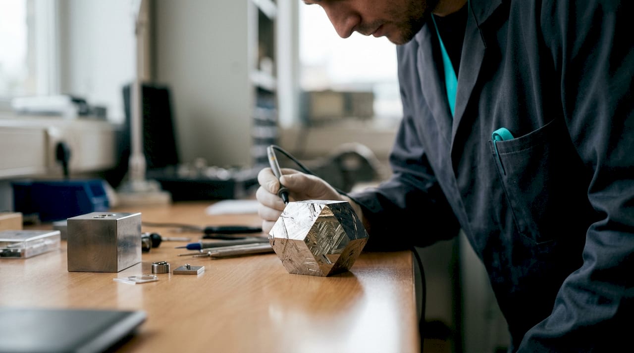
Hexagonally close-packed metals are the clearest example. The crystalline array in these metals allows scattering rates to differ along different lattice directions, so electrons traveling along the six-fold axis encounter a different environment than those moving perpendicular to it. The result is measurable conductivity variation between axes, even in a pure, defect-free crystal.
Microstructure adds another layer. Processing methods such as rolling, drawing, and 3D printing can induce crystallographic texture in materials that start out isotropic, creating preferred grain orientations that translate directly into directional transport properties. A rolled aluminum sheet and a cast aluminum block of identical composition can have meaningfully different thermal conductivity profiles simply because of how the grains are aligned. Grain boundaries in low-symmetry semiconductors can amplify anisotropy further, as research on β-Ga₂O₃ shows: oriented low-angle grain boundaries along the b-direction raise energy barriers up to 93 meV, pushing conductivity anisotropy well beyond what the intrinsic crystal structure alone would predict.
Real materials that show strong directional conductivity differences
Concrete numbers make the concept stick. Three materials illustrate the range of anisotropic behavior engineers actually encounter.
Cadmium (electrical): In this hexagonally close-packed metal, electrical conductivity runs at 1.3×10⁷ S/m along the six-fold axis and 1.5×10⁷ S/m perpendicular to it. The ratio is modest, but it is measurable and real, and it comes entirely from crystal symmetry.
Graphite (electrical): The contrast here is dramatic. Delocalized electrons move freely within the hexagonal carbon planes, but conduction perpendicular to those planes is roughly three orders of magnitude smaller. Graphite is one of the most anisotropic electrical conductors in common use, and its thermal conductivity and thermal expansion follow the same directional pattern.
Quartz (thermal): Thermal conductivity perpendicular to the c-axis measures 6.5 W/mK, while the value parallel to the c-axis reaches 11.3 W/mK. That nearly 2x difference in a single-crystal mineral explains why quartz cut parallel versus perpendicular to its c-axis spreads heat in visibly different elliptical patterns when heated from a point source.
Additional examples worth knowing:
Polymer thin films: Anisotropic thermal conductivity in these films is exploited in solid-state transducers and microelectronic packaging, where controlling heat flow direction is as important as the total conductance.
High-temperature superconductors like BiSrCaCuO: Superconducting pathways exist within the copper-oxide ab-planes but not perpendicular to them, a direct consequence of planar crystal anisotropy.
Sedimentary rock formations: Electrical conductivity parallel to layering differs from that perpendicular to it, a property the oil and gas industry uses to identify hydrocarbon-bearing sands from shale sequences.
How tensors mathematically capture directional conductivity
A scalar cannot represent anisotropic conductivity. A single number implies the same response in every direction, which is precisely what anisotropic materials contradict. The correct mathematical object is a second-rank tensor, which relates two vector quantities: the applied stimulus (electric field E or temperature gradient ∇T) and the resulting flux (current density J or heat flux q).
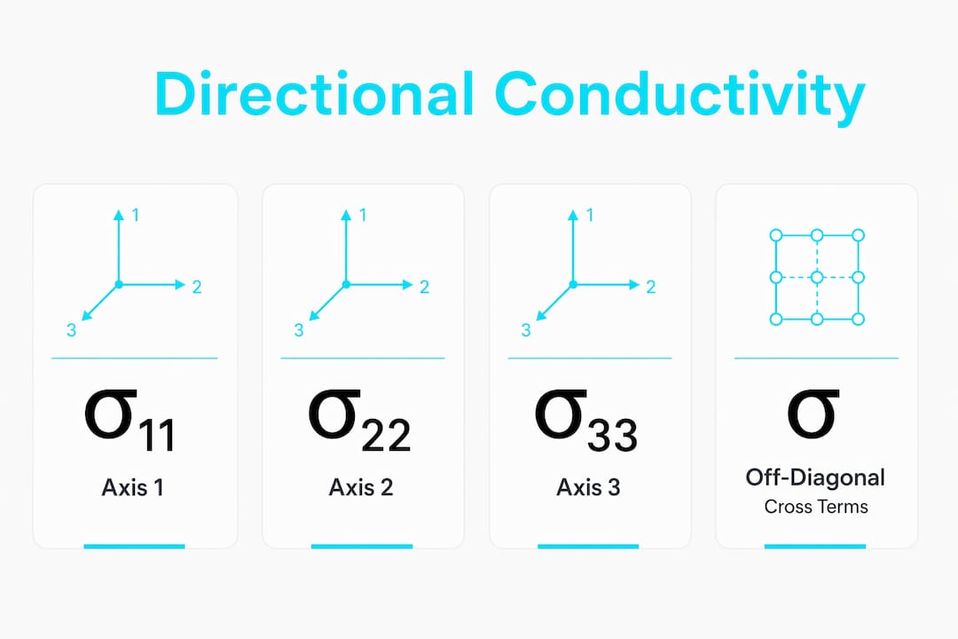
The conductivity tensor σ is written as a 3×3 matrix:
J_i = σ_ij · E_j
Each element σ_ij describes how a field component along direction j drives current along direction i. In the principal coordinate system, the off-diagonal elements vanish and the tensor reduces to three independent diagonal values: σ₁₁, σ₂₂, and σ₃₃ along the principal axes.
Key insight: In an anisotropic material, the current density vector J is generally not parallel to the electric field E. The off-diagonal tensor elements are what cause this misalignment. Ignoring them and treating conductivity as a scalar is not a conservative simplification; it is a modeling error that propagates into every downstream calculation.
Tensor element | Physical meaning |
σ₁₁, σ₂₂, σ₃₃ | Conductivity along each principal axis |
Off-diagonal σ_ij (i ≠ j) | Coupling between perpendicular field and flux components |
Principal axes | Directions where flux and gradient are parallel |
Tensor diagonalization | Rotation to principal frame eliminates off-diagonal terms |
The conductivity ellipsoid gives this a geometric face. Each semi-axis of the ellipsoid equals the conductivity magnitude along that principal direction. A sphere means isotropic; any deviation from spherical means anisotropic. For β-Ga₂O₃, van der Pauw measurements show the off-diagonal element is approximately 5% of the diagonal values, and the direction of highest conductivity sits rotated (59 ± 15)° from the c-direction.
How to measure anisotropic conductivity accurately
Standard four-probe or steady-state methods work fine for isotropic materials. For anisotropic ones, you need techniques that can resolve the full tensor, not just a single directional value.
Van der Pauw technique (electrical): Adapted for tensor measurements by using well-defined square sample geometries on differently oriented crystal faces. Comparing results from multiple surface orientations lets you extract the ratio of all tensor components. For β-Ga₂O₃, this approach resolved diagonal elements that deviate by no more than 6% from each other at room temperature, along with the off-diagonal element.
Beam-offset frequency-domain thermoreflectance (BO-FDTR): The thermal analog for low-symmetry materials. A pump laser heats the surface; a spatially offset probe laser measures the thermoreflectance response. By varying the offset direction and fitting to a heat transport model, you extract individual tensor components of thermal conductivity. This method is particularly valuable for materials lacking in-plane symmetry, where simpler techniques cannot distinguish between tensor components.
Finite-element simulation cross-validation: Experimental measurements alone rarely confirm tensor values without ambiguity. Pairing van der Pauw or BO-FDTR data with finite-element models of the exact sample geometry closes that gap. The simulation predicts the expected voltage or temperature distribution for a given tensor; discrepancies between simulation and measurement reveal off-diagonal contributions or geometric errors.
Ferroelectric switching for active control: In certain ferroelectric semiconductors, the conductivity tensor can be switched by polarization reversal, giving researchers a way to modulate anisotropy electrically rather than just measure it passively. This opens the door to devices where directional conductivity is a tunable parameter.
Pro Tip: When preparing van der Pauw samples from low-symmetry crystals, contact placement geometry is not a minor detail. Even small offsets from the ideal square geometry introduce systematic errors in the extracted off-diagonal tensor elements. Finite-element pre-simulation of your specific contact geometry before measurement saves significant time in data interpretation.
For engineers modeling anisotropic heat transfer in complex systems, understanding which measurement method produced the tensor data in your material database is as important as the values themselves.
Why anisotropic conductivity shapes engineering design decisions
Assuming isotropic conductivity in composites and textured metals is one of the most common modeling errors in thermal and electrical design. The consequences range from inaccurate temperature predictions to premature device failure.
Practical implications for engineering teams:
Thermal management: In fiber-reinforced composites, heat spreads preferentially along fiber axes. Designing a heat sink path without accounting for this directionality can leave hot spots exactly where the fibers do not run.
Semiconductor reliability: Anisotropic electrical conductivity in wide-bandgap semiconductors like β-Ga₂O₃ affects current crowding and breakdown behavior. Device layouts that ignore tensor orientation concentrate current in unintended directions.
Material selection: When two materials have similar bulk thermal conductivity values, their tensor profiles can differ enough to make one far better suited to a directional heat-spreading application than the other.
Numerical simulation accuracy: Finite-element thermal and electrical solvers accept full tensor inputs. Using a scalar approximation when tensor data is available discards information that the solver could use to produce a more accurate result.
Composite processing control: Rolling direction, fiber layup angle, and print orientation all shift the conductivity tensor. Specifying these parameters in manufacturing drawings is as important as specifying the material grade.
For EV battery thermal design, anisotropic conductivity in electrode materials and separator films directly affects how heat distributes across a cell under load, which in turn drives cell-to-cell temperature gradients at the pack level.
Structural engineers working with anisotropic materials in load-bearing applications face analogous challenges; lateral load distribution in composite panels, for instance, depends on the same directional property framework that governs thermal and electrical transport.
How temperature changes anisotropic conductivity
Temperature does not affect all tensor components equally, and that asymmetry matters for any device that operates across a wide temperature range. In β-Ga₂O₃, the conductivity anisotropy between the a and b directions stays within 2% for both dominant phonon scattering and dominant ionized-impurity scattering regimes. But the c-direction conductivity shifts from 0.96× the b-direction value under phonon scattering to 1.12× under ionized-impurity scattering. The dominant scattering mechanism changes with temperature and doping, so the tensor itself changes shape as the device heats up.
For metals, phonon scattering increases with temperature, generally reducing conductivity in all directions. But because scattering rates along different crystallographic axes respond differently to thermal excitation, the anisotropy ratio can grow or shrink with temperature rather than staying fixed. This means a material characterized at room temperature may behave quite differently at operating temperature, and thermal simulations that use room-temperature tensor values for a device running at elevated temperatures will carry that error through every result.
How anisotropic conductivity shapes material selection
Directional conductivity is a selection criterion, not just a material property to record. When the application demands heat spreading in one plane while blocking it in another, an anisotropic material is not a complication to work around; it is the solution. Pyrolytic graphite, for example, is chosen specifically because its in-plane thermal conductivity far exceeds its through-plane value, making it ideal for lateral heat spreading in compact electronics.
The selection process should start with the tensor, not the scalar average. Two materials with identical isotropic-equivalent conductivity can have completely different principal-axis profiles. One might spread heat uniformly; the other might channel it along a single axis. Matching the tensor geometry to the heat flow geometry of the application is what separates a good thermal design from one that merely passes a bulk conductivity spec.
For simulation-driven selection, tools that accept full tensor inputs rather than scalar approximations give you the ability to compare materials on the basis of directional performance. Jewlztech’s Thermalysis Toolkit supports variable material properties across a wide temperature range, making it practical to evaluate anisotropic candidates under realistic operating conditions rather than single-point assumptions.

Key Takeaways
Anisotropic conductivity requires tensor representation, directional measurement, and explicit modeling to avoid systematic errors in thermal and electrical design.
Point | Details |
Tensor, not scalar | Conductivity in anisotropic materials is a second-rank tensor; a scalar approximation discards directional information the solver could use. |
Crystal symmetry controls anisotropy | Cubic crystals are typically isotropic; hexagonal and monoclinic structures produce measurable conductivity differences between axes. |
Quartz thermal example | Quartz thermal conductivity runs 6.5 W/mK perpendicular to the c-axis and 11.3 W/mK parallel to it, nearly a 2x difference. |
Measurement method matters | Van der Pauw and BO-FDTR techniques resolve full tensor components; standard scalar methods cannot distinguish off-diagonal contributions. |
Temperature shifts the tensor | Dominant scattering mechanism changes with temperature, so the anisotropy ratio between axes can grow or shrink across the operating range. |
Recommended
Comments