
Thermal Radiation Calculation: Formulas and Examples for Engineers

For most engineering problems, three formulas cover the majority of thermal radiation calculations. A single isolated surface emits P = ε σ A T⁴, where σ = 5.67 × 10⁻⁸ W/(m² · K⁴) is the Stefan–Boltzmann constant. Net exchange between two black surfaces with a known view factor uses Q̇ = σ A₁ F₁₂ (T₁⁴ − T₂⁴). For real gray surfaces in an enclosure, you need surface emissivities and a radiosity balance. Everything else — participating gases, spectral coatings, and complex multi-surface enclosures — builds on these three starting points.
Which formula applies to your problem:
Single surface, no surroundings: P = ε σ A T⁴. Use this for a quick power estimate on a heated plate or electronic component radiating to a large cold environment.
Two-surface exchange, known geometry: Q̇ = σ A₁ F₁₂ (T₁⁴ − T₂⁴) for black bodies; add emissivity correction terms for gray surfaces.
Multi-surface enclosure (3+ surfaces, diffuse-gray): Set up the radiosity matrix and solve the linear system.
Gas-filled or combustion environments: Solve the Radiative Transfer Equation (RTE) with a participating-media solver.
For spreadsheet-based workflows, the Thermalysis Toolkit from Jewlztech handles all three surface-exchange modes with a built-in property database, so you can prototype and verify without writing solver code from scratch.
Key Takeaways
Accurate thermal radiation calculation requires matching the right formula to the problem geometry, surface properties, and medium — then verifying with limiting-case checks before finalizing any design number.
Point | Details |
Start with the right formula | Use P = ε σ A T⁴ for single surfaces; add view factors and emissivity terms for two-surface or enclosure exchange. |
Escalate to radiosity for 3+ surfaces | Set up the radiosity matrix and solve the linear system; the two-surface formula does not generalize to multi-surface enclosures. |
Use h_rad ≈ 4 ε σ T_ref³ for small ΔT | The linearized coefficient is accurate within a few percent when ΔT / T_ref is below roughly 10%. |
Always verify with limiting cases | Set ε → 1 and check against the blackbody limit; confirm energy balance sums to zero in closed enclosures. |
Jewlztech Thermalysis Toolkit | Spreadsheet-based radiation module with built-in property database; supports single-surface, two-surface, and multi-surface radiosity workflows. |
Table of Contents
Core equations every engineer needs for radiative heat transfer
How view factors work and how to compute them for real geometries
Setting up the radiosity method for multi-surface enclosures
Linearizing radiation into an effective heat transfer coefficient
Practical tools, calculators, and data sources for radiation problems
A compact checklist for setting up any radiation calculation
What actually matters in radiation calculations (and what engineers get wrong)
The Thermalysis Toolkit handles radiation calculations from prototype to enclosure
When thermal radiation matters in engineering analysis
Thermal radiation is electromagnetic energy emitted by any surface above absolute zero. Unlike conduction or convection, it requires no medium — radiation transfers heat across a vacuum just as readily as through air. The governing physics ties emission to the fourth power of absolute temperature, which means radiation grows fast: double the temperature and emission increases by a factor of sixteen.
Situations where you must include radiation in your heat balance:
Surface temperatures above roughly 300°C, where radiative flux becomes comparable to or larger than convective flux
Vacuum or low-pressure environments (spacecraft, vacuum furnaces) where convection is negligible
Furnaces, kilns, and combustion chambers where radiation is the dominant transfer mode
Steady-state energy balances for structures exposed to solar flux or cryogenic surroundings
Optical and infrared systems where spectral emission matters
Blackbody vs. gray body — the practical distinction:
A blackbody is an idealized perfect emitter and absorber: emissivity ε = 1 at all wavelengths.
A gray body has ε < 1 but constant across wavelengths — the standard engineering approximation for metals and many coatings.
Real surfaces are spectrally selective: emissivity varies with wavelength. For precision work (solar absorbers, cryogenic shields, infrared sensors), you need spectral emissivity data rather than a single total value.
When combining radiation with conduction and convection, the heat transfer modeling workflow matters as much as the individual formulas.
Core equations every engineer needs for radiative heat transfer
Stefan–Boltzmann law
For a gray, opaque surface:
P = ε σ A T⁴
where ε is total hemispherical emissivity (0 < ε ≤ 1), σ = 5.67 × 10⁻⁸ W/(m² · K⁴), A is surface area in m², and T is absolute temperature in Kelvin. Always use Kelvin. Plugging in Celsius is the single most common numerical error in radiation problems.
Planck’s law and Wien’s displacement law
When spectral behavior matters, Planck’s law gives the spectral emissive power of a blackbody as a function of wavelength and temperature. Wien’s displacement law locates the peak wavelength: λ_max T = 2898 μm · K. At 1000 K, peak emission sits near 2.9 μm (mid-infrared); at 5800 K (the Sun’s effective surface), near 0.5 μm (visible). Use these when surface coatings or detector windows are wavelength-selective.
Net exchange formulas
For two black surfaces with view factor F₁₂:
Q̇₁₂ = σ A₁ F₁₂ (T₁⁴ − T₂⁴) (where σ is the Stefan–Boltzmann constant).
For two gray, diffuse, opaque surfaces forming a complete enclosure (the two-surface gray enclosure formula):
Q̇₁₂ = σ (T₁⁴ − T₂⁴) / [ (1−ε₁)/(ε₁A₁) + 1/(A₁F₁₂) + (1−ε₂)/(ε₂A₂) ]
The denominator terms represent surface resistance (from emissivity) and geometric resistance (from view factor). This structure generalizes directly to the radiosity network for larger enclosures.
Assumptions embedded in these formulas:
Surfaces are isothermal and opaque
Emission is diffuse (Lambert’s cosine law holds)
Emissivity is wavelength-independent (gray approximation)
The medium between surfaces is non-participating (transparent)
Unit consistency is non-negotiable: area in m², temperature in K, emissivity dimensionless. The result is in watts. As Howell et al. document in their foundational Thermal Radiation Heat Transfer reference, these surface-exchange formulations underpin both hand calculations and numerical radiosity solvers.
How view factors work and how to compute them for real geometries
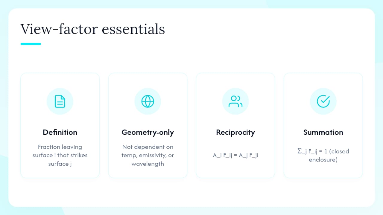
A view factor F_ij is the fraction of radiation leaving surface i that strikes surface j directly. It depends purely on geometry — not on temperature, emissivity, or wavelength. That geometry-only property is what makes view factors reusable across different operating conditions for the same physical configuration.
Two rules govern every view-factor calculation, as established in standard radiation view factor references:
Reciprocity: A_i F_ij = A_j F_ji
Summation (closure): Σⱼ F_ij = 1 for every surface i in a closed enclosure
These two rules let you derive unknown view factors algebraically once you know a subset of them — often eliminating the need for numerical integration on several surfaces.
Analytic formulas for common geometries
Closed-form expressions exist for a useful set of configurations:
Two large parallel plates of equal area: F₁₂ = 1 (all radiation from plate 1 reaches plate 2)
Coaxial parallel disks: analytic formula involving radius ratio and separation distance, available in view factor catalogs
Concentric cylinders or spheres: F_inner→outer = 1 by geometry
Plate to adjacent perpendicular plate: closed-form result from the crossed-string method
When geometry departs from these standard cases, you need numerical methods.
Computational methods for complex geometries
Crossed-string (Hottel) method: exact for 2D geometries; fast and requires only string lengths between surface edges
Hemicube projection: projects hemisphere of directions onto a unit cube face; standard in rendering and radiation codes
Numerical integration: direct integration of the double-area integral over surface pairs; accurate but expensive for large meshes
Mesh-based routines: tools like the TNSolver view-factor scripts automate this for many standard configurations in MATLAB/Octave
Pro Tip: Subdivide large or concave surfaces into smaller patches before computing view factors. Concave surfaces can “see themselves” (F_ii > 0), and a coarse mesh misses that self-irradiation. After subdividing, use reciprocity and the summation rule to recover the remaining factors algebraically — this cuts numerical integration effort significantly without sacrificing accuracy.
Setting up the radiosity method for multi-surface enclosures
When three or more diffuse-gray surfaces exchange radiation, the two-surface formula no longer applies directly. The radiosity method handles this by writing an energy balance for each surface and solving the resulting linear system.
Radiosity J_i is the total radiation leaving surface i per unit area: emitted plus reflected. For a diffuse-gray surface:
J_i = ε_i σ T_i⁴ + (1 − ε_i) G_i
where G_i is the irradiation (total incoming flux) on surface i.
Setting up the system — step by step:
Define N surfaces, each with known area A_i, emissivity ε_i, and temperature T_i (or net heat flux, if temperature is unknown).
Write the irradiation on each surface as a weighted sum of radiosities from all other surfaces: G_i = Σⱼ F_ij J_j.
Substitute into the radiosity definition to get N equations in N unknowns (the J_i values).
Arrange as a matrix equation: [M]{J} = {b}, where M contains the geometric conductance terms A_i F_ij and emissivity factors, and b contains the blackbody emission terms ε_i σ T_i⁴.
Solve with LU decomposition, numpy.linalg.solve in Python, or the backslash operator in MATLAB/Octave.
Recover net heat transfer at each surface: Q_i = A_i (J_i − G_i).
For a 3-surface enclosure, the matrix is 3×3 and easily solved by hand or in a spreadsheet. For larger enclosures (furnace walls, solar receivers, thermal-control panels), the same structure scales directly — only the matrix size grows. The UC Merced radiative heat transfer notes provide applied guidance on assembling and solving these systems for engineering enclosures.
When to use radiosity vs. the two-surface formula:
Use the two-surface gray enclosure formula when exactly two surfaces dominate the exchange and the geometry is simple. Switch to the radiosity matrix as soon as a third surface participates meaningfully, or when you need the net flux at each individual surface rather than just the total exchange.
Participating media and when to escalate to RTE solvers
If the space between surfaces contains a gas that absorbs, emits, or scatters radiation — combustion products, steam, CO₂, soot — the transparent-medium assumption fails. Radiation interacts with the volume, not just the bounding surfaces, and you need the Radiative Transfer Equation.
The RTE describes how intensity changes along a ray path through the medium:
dI/ds = −(κ + σ_s) I + κ I_b + (σ_s / 4π) ∫ I Φ dΩ
where κ is the absorption coefficient, σ_s the scattering coefficient, I_b the blackbody intensity, and Φ the scattering phase function. As UC Merced’s engineering notes point out, the RTE is a 6-dimensional problem in space and direction, which is why it demands dedicated solvers rather than spreadsheet arithmetic.
Practical solver options:
Discrete Ordinates Method (DOM/S_N): discretizes the angular domain into a finite set of directions; widely implemented in CFD codes; good balance of accuracy and cost
P-1 approximation: simplifies angular dependence to a diffusion-like equation; fast but loses accuracy for optically thin media or strong anisotropic scattering
Monte Carlo ray tracing: statistically exact; handles complex geometry and spectral variation well; computationally expensive but parallelizes easily
Line-by-line (LBL) and k-distribution methods: high-accuracy spectral models for gas mixtures; used when CO₂/H₂O band structure matters (combustion, atmospheric radiation)
As Modest’s Radiative Heat Transfer details, choosing among these methods depends on optical thickness, scattering importance, geometric complexity, and available compute budget.
Quick decision checklist:
Optical thickness τ = κ L < 0.1: medium is nearly transparent; surface-only radiosity is adequate
τ > 1: medium is optically thick; P-1 or DOM is appropriate
Strong scattering (σ_s comparable to κ): avoid P-1; use DOM or Monte Carlo
Complex 3D geometry with soot or particles: Monte Carlo or DOM in a CFD framework
High-accuracy spectral work (combustion, atmospheric): LBL or k-distribution
Linearizing radiation into an effective heat transfer coefficient
For problems where the temperature difference between surfaces is small relative to the mean temperature, you can linearize the T⁴ dependence and treat radiation as an equivalent convective coefficient. This lets you combine radiation with convection and conduction in a single thermal resistance network.
Starting from the net exchange between a gray surface and its surroundings:
Q̇ = ε σ A (T_s⁴ − T_surr⁴)
Factor the difference of fourth powers:
T_s⁴ − T_surr⁴ = (T_s² + T_surr²)(T_s + T_surr)(T_s − T_surr)
Define T_ref as the mean temperature (T_s + T_surr)/2. For small ΔT, the first three factors collapse approximately to 4 T_ref³, giving:
h_rad ≈ 4 ε σ T_ref³
Net radiative flux then becomes Q̇ ≈ h_rad A (T_s − T_surr), directly addable to convective flux.
When linearization holds and when it breaks down:
Acceptable when ΔT / T_ref < 0.1 (roughly 10% temperature swing around the mean); error stays within a few percent
Breaks down for furnace or combustion conditions where ΔT is hundreds of degrees and T_ref is itself uncertain
Useful for electronics cooling estimates, building envelope calculations, and combined-mode hand calculations where a quick check is needed before running a full solver
For a combined-mode heat transfer techniques guide, h_rad sits in parallel with h_conv in the thermal resistance network, and the total surface coefficient is simply h_total = h_conv + h_rad.
Worked step-by-step calculations you can reproduce
Example 1: Two large parallel plates
Setup: Two large parallel plates, each 1 m², facing each other. Plate 1 at T₁ = 800 K, ε₁ = 0.8. Plate 2 at T₂ = 400 K, ε₂ = 0.6. Find net radiative heat transfer from plate 1 to plate 2.
Step 1 — View factor. For two large parallel plates of equal area, F₁₂ = 1.
Step 2 — Gray enclosure formula.
Q̇₁₂ = σ (T₁⁴ − T₂⁴) / [ (1−ε₁)/(ε₁A₁) + 1/(A₁F₁₂) + (1−ε₂)/(ε₂A₂) ]
Denominator terms:
(1 − 0.8)/(0.8 × 1) = 0.25
1/(1 × 1) = 1.00
(1 − 0.6)/(0.6 × 1) = 0.667
Total denominator = 1.917 m⁻²
Numerator: σ(T₁⁴ − T₂⁴) = 5.67 × 10⁻⁸ × (800⁴ − 400⁴) = 5.67 × 10⁻⁸ × (4.096 × 10¹¹ − 2.56 × 10¹⁰) = 5.67 × 10⁻⁸ × 3.84 × 10¹¹ = 21,773 W/m²
Q̇₁₂ = 21,773 / 1.917 ≈ 11,358 W
Sanity check: The blackbody limit (ε₁ = ε₂ = 1) gives 21,773 W. Gray-body result is lower, as expected. Use the Omni Stefan–Boltzmann calculator to verify the numerator independently.
Example 2: Three-surface enclosure via radiosity matrix
Setup: A triangular enclosure with three diffuse-gray surfaces. A₁ = A₂ = A₃ = 1 m². ε₁ = 0.9, ε₂ = 0.7, ε₃ = 0.5. T₁ = 1000 K, T₂ = 600 K, T₃ = 300 K. View factors for an equilateral triangular enclosure: F₁₂ = F₁₃ = F₂₃ = 0.5 (by symmetry and summation rule).
Step 1 — Blackbody emissive powers.
E_b1 = σ × 1000⁴ = 56,700 W/m²
E_b2 = σ × 600⁴ = 7,348 W/m²
E_b3 = σ × 300⁴ = 459 W/m²
Step 2 — Surface resistance terms (1 − εᵢ)/(εᵢ Aᵢ):
R_s1 = 0.1/0.9 = 0.111
R_s2 = 0.3/0.7 = 0.429
R_s3 = 0.5/0.5 = 1.000
Step 3 — Geometric resistance terms 1/(Aᵢ Fᵢⱼ) = 1/(1 × 0.5) = 2.0 for all pairs.
Step 4 — Matrix structure. The radiosity balance for surface 1:
(J₁ − E_b1)/R_s1 = (J₁ − J₂)/2.0 + (J₁ − J₃)/2.0
Rearranging all three surfaces produces a 3×3 linear system. Solve with a matrix solver (numpy, MATLAB, or a spreadsheet solver). The resulting radiosities J₁, J₂, J₃ then give net heat transfer at each surface via Q_i = (E_bi − J_i)/R_si.
Unit check: All areas in m², temperatures in K, σ in W/(m² · K⁴). Result in watts.
Reproduce this in a spreadsheet or load the geometry into the Thermalysis Toolkit radiation module to verify your matrix assembly and solution.
Practical tools, calculators, and data sources for radiation problems
The right tool depends on problem complexity. A quick single-surface estimate needs nothing more than a calculator. A 20-surface furnace enclosure with participating gases needs a dedicated solver.
Task | Recommended tool | Key inputs needed |
Single-surface emission estimate | Omni Stefan–Boltzmann calculator | ε, A, T |
Two-surface gray exchange | Engineering Toolbox radiation calculator | ε₁, ε₂, A₁, F₁₂, T₁, T₂ |
View factor lookup (standard geometry) | Thermalradiation.net catalog | Geometry type, dimensions |
View factor computation (custom geometry) | TNSolver MATLAB/Octave scripts | Surface mesh, coordinates |
Multi-surface radiosity (3–20 surfaces) | Thermalysis Toolkit / custom spreadsheet | Aᵢ, εᵢ, Fᵢⱼ, Tᵢ |
RTE / participating media | OpenFOAM (DOM), ANSYS Fluent, Radiance | κ, σ_s, geometry, boundary conditions |
Data sources for emissivity and material properties:
NIST — is the authoritative source for thermophysical and optical property data. The NIST WebBook provides emissivity and spectral property data for metals, oxides, and coatings across temperature ranges relevant to engineering.
Modest’s Radiative Heat Transfer (Elsevier) includes extensive spectral emissivity tables and gas-property data for participating-media calculations
For a broader look at how radiation tools fit into a full simulation workflow, the CFD software alternatives guide covers solver options when you need to move beyond spreadsheet radiosity.
Common mistakes that corrupt radiation calculations
Unit errors:
Using Celsius instead of Kelvin in T⁴ terms — this is catastrophic, not a small perturbation. 100°C = 373 K; 100⁴ vs. 373⁴ differ by a factor of nearly 200.
Mixing cm² and m² for area when emissivity data is quoted per cm².
Forgetting that σ = 5.67 × 10⁻⁸ W/(m² · K⁴) — not per cm² or per ft².
Emissivity misuse:
Confusing total hemispherical emissivity (what the formulas use) with normal spectral emissivity (what many measurement reports give). They can differ by 20–30% for metals.
Applying a room-temperature emissivity value at 800 K, where surface oxidation and spectral shifts change ε significantly.
Treating a polished metal (ε ≈ 0.05) as a gray body when its emissivity rises sharply with temperature.
Over-applying the blackbody assumption:
Setting ε = 1 for a quick estimate is fine for order-of-magnitude work, but never for design decisions on surfaces with coatings, oxidation, or selective emitters.
Assuming F₁₂ = 1 for surfaces that are not large, parallel, and directly facing — even a modest angular offset drops F₁₂ well below 1.
Verification shortcuts that catch errors fast:
Limiting-case check: set ε → 1 and verify the result matches the blackbody formula. Set F₁₂ → 0 and confirm Q̇ → 0.
Energy balance: net heat leaving all surfaces in a closed enclosure must sum to zero (or to the net power input if one surface is heated).
Linearization cross-check: compute h_rad ≈ 4 ε σ T_ref³ and multiply by A ΔT. If this rough estimate disagrees with your full calculation by more than ~15%, recheck your view factors or emissivity values.
A compact checklist for setting up any radiation calculation
Follow this sequence before running numbers or code. Skipping steps early creates errors that are hard to trace later.
Define control surfaces. List every surface that participates in the exchange. Assign area, temperature (or heat flux), and emissivity to each. Decide whether the enclosure is closed or open.
Choose gray vs. spectral. If surfaces are coated, selective, or the problem involves solar flux and infrared re-emission, you need spectral emissivity data. For most industrial surfaces at uniform temperature, the gray approximation is adequate.
Obtain emissivity values. Pull from NIST, Modest, or Howell tables. Note the temperature range and measurement geometry (total hemispherical preferred).
Compute or look up view factors. Use analytic formulas for standard geometries. Apply reciprocity and summation to fill the view-factor matrix. Verify that each row sums to 1.
Choose your solver. Two surfaces and simple geometry: use the two-surface gray enclosure formula. Three or more diffuse-gray surfaces: set up the radiosity matrix. Participating media: select DOM, P-1, or Monte Carlo based on optical thickness and geometry.
Assemble inputs and run. For radiosity, build the matrix and solve. For RTE, set boundary conditions, mesh, and solver tolerances.
Verify results. Run limiting-case checks (ε → 1, F → 0 or 1). Check energy balance. For numerical solvers, test mesh refinement — if the answer changes more than a few percent on refinement, the mesh is too coarse.
Document assumptions. Record the emissivity source, view-factor method, solver settings, and any simplifications (gray approximation, closed enclosure, non-participating medium). This is what makes a calculation reproducible and defensible in a design review.
For a broader heat transfer applications reference covering furnaces, solar receivers, and electronics, the same checklist applies with problem-specific geometry inputs.
What actually matters in radiation calculations (and what engineers get wrong)
Most radiation errors in practice are not formula errors. They are assumption errors: someone applied the two-surface formula to a five-surface enclosure, or used a room-temperature emissivity at 700 K, or forgot that a concave surface sees itself. The formulas are not the hard part.
The harder discipline is knowing when to escalate. A linearized h_rad is genuinely useful for electronics cooling or building envelope estimates — it gets you within a few percent with almost no effort when ΔT is modest. But applying that same linearization to a furnace wall at 1200 K with a 600 K temperature swing produces results that are wrong by a factor, not a percentage. The T⁴ dependence is not a detail to linearize away when the temperature ratio is large.
View factors deserve more attention than most engineers give them. The reciprocity and summation rules are not just mathematical conveniences — they are the primary tool for reducing a complex geometry to a tractable set of unknowns. An engineer who can apply the crossed-string method or subdivide a surface intelligently will spend far less time on numerical integration than one who reaches for a mesh-based solver for every problem.
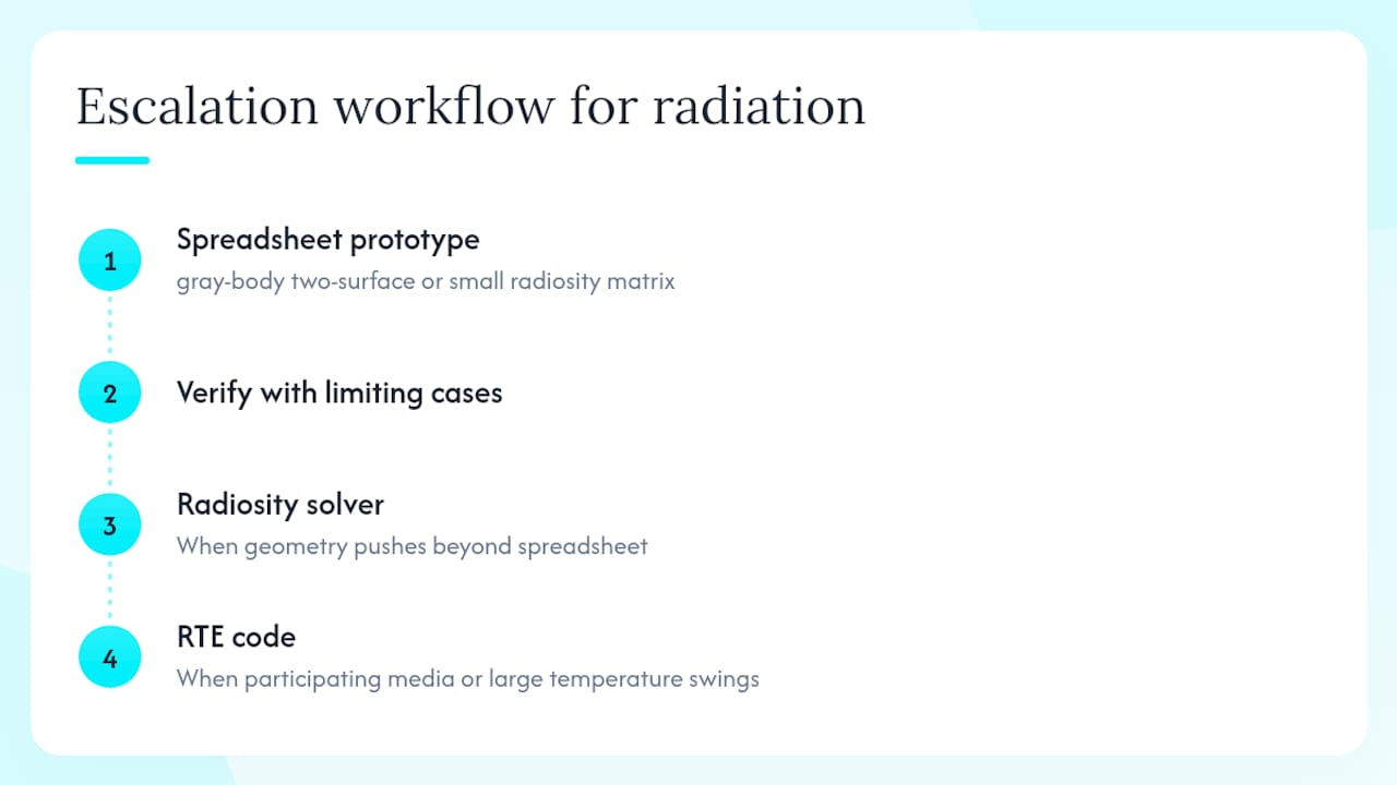
The workflow that holds up across problem types: start with a spreadsheet prototype using the gray-body two-surface formula or a small radiosity matrix. Verify with limiting cases. If the geometry or participating media push beyond what the spreadsheet handles cleanly, move to a radiosity solver or RTE code. That progression — hand calculation to radiosity to RTE — keeps you from over-engineering simple problems while still catching the cases where a simple formula genuinely fails.
The Thermalysis Toolkit handles radiation calculations from prototype to enclosure
Jewlztech built the Thermalysis Toolkit specifically for engineers who want spreadsheet-based radiation workflows without writing solver code from scratch. The toolkit covers single-surface emission, two-surface gray exchange, and multi-surface radiosity calculations, with a built-in material property database that pulls emissivity values directly into your worksheet.

Students prototyping the worked examples in this article can load geometry and emissivity inputs directly into the radiation module and compare results against their hand calculations. Practicing engineers get repeatable, documented worksheets for enclosure problems — the kind of calculation that needs to be auditable in a design review. The free version covers core conduction, convection, and radiation estimates. Upgrading to the paid subscription adds advanced radiosity solver support, larger geometry configurations, and built-in spectral property data for higher-temperature applications. Try the Thermalysis Toolkit at the link above and run the parallel-plate example from this article as your first verification case.
Sources
The references below are where the formulas in this article come from and where to go when a problem exceeds what a spreadsheet handles.
Recommended
Comments