
Heat Transfer Model: Engineering Guide to Methods and Math


A heat transfer model is a mathematical or numerical framework governed by the heat equation — a partial differential equation (PDE) — that predicts temperature distributions and heat flux in physical systems by combining conduction, convection, and radiation.
Three things worth knowing before you go further:
Transient vs. steady-state: If temperatures change over time (startup, cool-down, cyclic loading), you need a transient model. If the system has reached thermal equilibrium, a steady-state formulation is faster and often sufficient.
When to couple with CFD: If the flow field significantly affects heat transfer (forced convection, turbulent jets, buoyancy-driven flows), a conjugate heat transfer simulation that solves momentum and energy equations together will outperform a simple convective boundary condition.
When lumped models suffice: For small, thermally conductive objects with a Biot number well below 0.1, the lumped capacitance method gives accurate transient results with almost no computational overhead.
Your next three steps after reading this guide:
Define your domain geometry and boundary conditions (BCs) — Dirichlet, Neumann, or Robin.
Choose your approach: analytical solution, finite-difference method (FDM), finite-element method (FEM), or finite-volume method (FVM).
Validate with at least one verification test before trusting your results.
Table of Contents
What governs a heat transfer model: the heat equation and boundary conditions
How conduction, convection, and radiation appear in your model
Analytical and semi-analytical models: when the math is enough
Conjugate heat transfer: when you need to solve the fluid too
Worked example: 1-D transient conduction from setup to validation
Thermalysis Toolkit by Jewlztech covers the full modeling workflow
What governs a heat transfer model: the heat equation and boundary conditions
The foundation of any thermal conduction model is the transient heat equation in conservation form:
ρ c_p (∂T/∂t) = ∇·(k ∇T) + q̇
where T is temperature (K or °C), ρ is density (kg/m³), c_p is specific heat capacity (J/kg·K), k is thermal conductivity (W/m·K), and q̇ is the volumetric heat generation rate (W/m³). For a single-layer homogeneous material, this transient conduction simplifies to ρ c_p (∂T/∂t) = k (∂²T/∂s²) along the spatial coordinate s.
Drop the time derivative and you get the steady-state form: ∇·(k ∇T) + q̇ = 0. That is the equation to solve when temperatures no longer change with time.
The heat equation is a statement of energy conservation. Every term has a physical meaning: the left side is the rate of energy storage in the material; the first right-side term is net conductive flux into a control volume; the second is internal heat generation. Lose sight of that and boundary conditions become arbitrary numbers rather than physical constraints.
Source terms deserve special attention. Volumetric, layer, and point heat sources are the three common types in PDE formulations, and localized mesh refinement near point or line sources is necessary to avoid large discretization errors.
Initial conditions (ICs) for transient problems specify T(x, 0) = T₀(x) everywhere in the domain. A uniform initial temperature is the most common assumption, but non-uniform ICs arise in restart analyses or when modeling a system that has already partially heated.
Boundary condition types determine how the domain interacts with its environment:
Dirichlet (Type I): Fixed temperature at the boundary, T = T_wall. Use this when a surface is held at a known temperature (isothermal wall, controlled bath).
Neumann (Type II): Specified heat flux, −k (∂T/∂n) = q″. A zero-flux (adiabatic) condition is the special case where q″ = 0.
Robin / convective (Type III): −k (∂T/∂n) = h(T − T_∞). This couples the surface temperature to an ambient fluid through a heat transfer coefficient h (W/m²·K).
The Fourier number, Fo = α t / L², where α = k/(ρ c_p) is thermal diffusivity, scales transient behavior. A small Fo means the system is still in early transient; Fo >> 1 means it has nearly reached steady state. Checking Fo before choosing a time-step size is a quick sanity check that saves debugging time later.
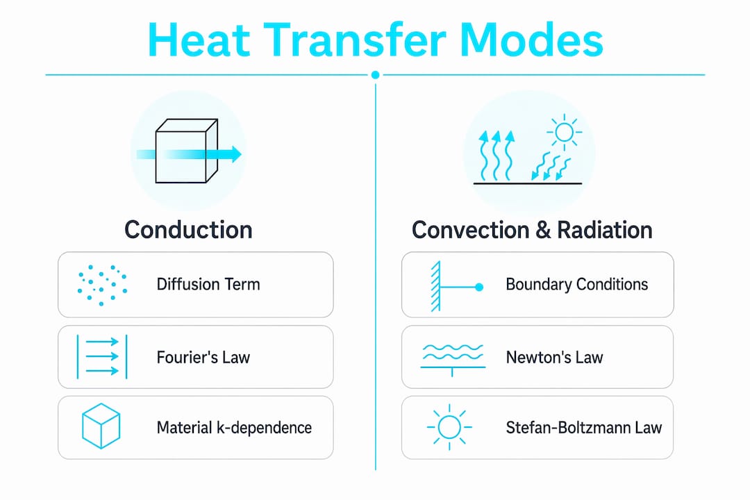
How conduction, convection, and radiation appear in your model
Each mode of heat transfer enters the governing equations differently, and choosing the right representation for each is where most modeling decisions are made.
Conduction appears as the diffusion term ∇·(k ∇T) in the heat equation. For isotropic materials, k is a scalar; for composites or crystals, it becomes a tensor. The steady-state closed-form result for a flat wall is Q = kA ΔT / L, which is the thermal equivalent of Ohm’s law and the basis for thermal resistance networks.
Convection enters in two ways. As a boundary condition (the Robin form above), it represents heat exchange with a fluid using a lumped coefficient h. As a volume phenomenon, it requires solving the Navier-Stokes momentum equations alongside the energy equation — that is conjugate heat transfer, covered in its own section below. The choice between these two representations depends on whether the flow field is known and uniform (use a BC) or spatially varying and coupled to the temperature field (use full CFD).
Radiation is the most nonlinear of the three modes. Surface emission follows the Stefan-Boltzmann law: q″_rad = ε σ T⁴, where ε is emissivity and σ = 5.67 × 10⁻⁸ W/m²·K⁴. For enclosures, the net radiative exchange between surfaces depends on view factors and the radiosity method.
Mode | Mathematical form | Dominant regime | Typical simplification |
Conduction | ∇·(k ∇T) | Solids, low-velocity fluids | Constant k, 1-D geometry |
Convection (BC) | h(T − T_∞) | Forced/natural convection surfaces | Uniform h from correlation |
Convection (full) | ρ u·∇T = ∇·(k ∇T) | Turbulent flow, buoyancy-driven | RANS turbulence model |
Radiation | ε σ (T⁴ − T_surr⁴) | High-T furnaces, space structures | Grey-diffuse surface |
Decision guidance by application:
Electronics cooling (< 150°C): Conduction dominates in the solid; convection BC with a correlation-based h is usually sufficient. Radiation is often negligible below 100°C.
Heat exchangers: Convection on both fluid sides plus conduction through the wall. A heat exchanger analysis using the NTU-effectiveness method can replace a full CFD model for preliminary design.
Furnaces and combustion chambers: Radiation dominates above roughly 800°C and cannot be treated as a correction term.
The grey-body, diffuse-surface assumption (ε independent of wavelength and direction) is acceptable for engineering metals at moderate temperatures. It breaks down for selective emitters like low-e coatings or for problems where spectral accuracy matters.
Pro Tip: Before adding radiation to a model, estimate the radiative heat flux using q″ = ε σ T⁴ and compare it to the convective flux q″ = h ΔT. If the radiative term is less than 5% of the convective term, you can safely drop it and save significant solver complexity.
Analytical and semi-analytical models: when the math is enough
Numerical methods are not always the right tool. For a surprising number of engineering problems, closed-form or semi-analytic solutions are faster, more transparent, and easier to validate.
Lumped capacitance is the simplest transient model. It treats the entire solid as a single node at uniform temperature T(t), giving:
T(t) − T_∞ = (T_i − T_∞) exp(−t / τ), where τ = ρ V c_p / (h A_s)
The assumption is valid when the Biot number Bi = h L_c / k < 0.1, where L_c = V/A_s is the characteristic length. When Bi is below that threshold, internal conduction resistance is negligible compared to surface convection resistance. Use this for small metal components cooling in air, thermocouple time-constant estimates, and quick first-pass transient estimates.
A caution worth noting: check Bi at multiple locations and for all relevant surface conditions. A single Biot calculation at a nominal condition can mislead you for assemblies with non-uniform heat transfer coefficients.
1-D transient solutions for infinite slabs, cylinders, and spheres are available as eigenfunction series (Heisler charts or their analytic equivalents). These assume:
Uniform initial temperature T_i
Constant surface temperature or constant h (Robin BC)
Constant, isotropic material properties
They are accurate for the first few terms of the series when Fo > 0.2. Below that, you need more terms or a numerical approach.
Steady-state analytical solutions cover a wide range of geometries:
Flat wall: Q = kA ΔT / L
Cylindrical wall: Q = 2πkL ΔT / ln(r_o/r_i)
Spherical shell: Q = 4πk r_i r_o ΔT / (r_o − r_i)
Composite walls: thermal resistances in series or parallel
Semi-analytic methods — separation of variables, eigenfunction expansions, Green’s functions — extend these to non-uniform BCs and multi-region domains. They remain practical when the geometry is regular (rectangular, cylindrical, spherical) and the BCs are separable. Once the geometry becomes irregular or material properties become temperature-dependent, the algebra grows intractable and numerical methods take over.
For phase-change problems, the picture changes entirely. Enthalpy-porosity, effective heat capacity, fixed-grid enthalpy, and moving-boundary (Stefan) approaches are the main phase-change model options, each with different accuracy-vs-complexity trade-offs. No simple closed-form solution exists for most practical PCM geometries.
Numerical methods: FDM, FEM, and FVM compared
When geometry is complex, properties are temperature-dependent, or the domain involves multiple coupled physics, numerical methods are the practical path forward.
Finite-difference method (FDM) discretizes the PDE on a structured grid by replacing derivatives with difference quotients. It is the easiest to implement from scratch, making it ideal for quick prototyping, 1-D and 2-D parametric studies, and teaching. Its weakness is structured-grid dependence — curved boundaries require special treatment.
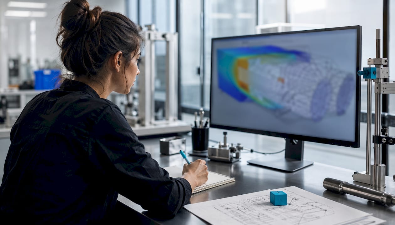
Finite-element method (FEM) divides the domain into elements (triangles, tetrahedra, quads, hexahedra) and solves a weak form of the PDE. It handles complex geometry and unstructured meshes naturally, which is why most commercial thermal simulation tools use it. The MOOSE framework’s Heat Transfer Module is a well-documented open-source FEM implementation that supports coupled thermal-mechanical and thermal-fluid problems.
Finite-volume method (FVM) integrates the conservation form of the PDE over control volumes, guaranteeing local and global energy conservation. This property makes FVM the dominant choice in CFD codes and the natural fit for conjugate heat transfer simulations where energy must be conserved across fluid-solid interfaces.
Time integration and stability
For transient problems, three time-integration schemes cover most practical needs:
Explicit (forward Euler): Simple but conditionally stable. The stability constraint is Fo ≤ 0.5 for 1-D FDM, which forces very small time steps for fine meshes or high-diffusivity materials.
Implicit (backward Euler): Unconditionally stable, but requires solving a linear system at each time step. Use this when stability, not accuracy, is the binding constraint.
Crank-Nicolson: Second-order accurate in time and unconditionally stable. The preferred choice for most transient heat transfer simulations when accuracy matters.
Stability and accuracy are not the same thing. An implicit scheme will not blow up, but it can still produce large temporal truncation errors if the time step is too coarse. Always verify that halving the time step does not change your results by more than your tolerance before trusting a transient solution.
Mesh strategy and convergence
Start with a coarse mesh, solve, then refine by a factor of 2 in each direction and solve again. If the temperature field changes by less than your target tolerance (typically 1–2% for engineering work), the coarser mesh is adequate. Concentrate refinement near:
Boundaries with high heat flux or steep gradients
Material interfaces with discontinuous conductivity
Point or line heat sources
Pro Tip: For convection-dominated problems, the boundary layer thickness δ should be resolved with multiple elements to capture gradients adequately. Skipping this step is a common cause of under-predicted heat transfer coefficients in FEM thermal models.
Solver choice matters at scale. For small to medium problems (< 10⁵ degrees of freedom), direct solvers (LU factorization, PARDISO) are reliable and fast. For large problems, iterative solvers (GMRES, conjugate gradient) with an ILU or algebraic multigrid preconditioner are necessary. Anisotropic conductivity and discontinuous material properties can stall iterative solvers — preconditioning becomes critical in those cases.
In extreme regimes, classical Fourier conduction breaks down entirely. In high-Knudsen-number or plasma environments, non-local transport models such as SNB outperform ad-hoc flux limiters. Most engineering problems operate outside this extreme regime, but it is worth knowing the boundary exists.
Conjugate heat transfer: when you need to solve the fluid too
Conjugate heat transfer (CHT) means solving the energy equation in both the solid and the fluid simultaneously, with the momentum equation governing the flow field. The solid conducts heat; the fluid carries it away. Neither can be solved independently when the flow structure significantly affects the temperature distribution.
When does CHT matter? Ask three questions:
Is the local Nusselt number Nu strongly position-dependent (entry-length effects, separated flow, jet impingement)? If yes, a uniform h BC will be wrong.
Is the Grashof number Gr large enough that buoyancy-driven flow is significant? Natural convection in enclosures often requires CHT.
Does the solid temperature distribution feed back into the fluid viscosity or density in a way that changes the flow? High-viscosity fluids and gases at large ΔT often do.
If any answer is yes, a convective BC calibrated by a bulk correlation will introduce meaningful error.
Practical CHT workflow:
Define separate solid and fluid domains with a shared interface.
Apply continuity conditions at the interface: temperature continuity (T_solid = T_fluid) and heat flux continuity (−k_s ∂T/∂n = −k_f ∂T/∂n).
Choose coupling strategy: one-way coupling (fluid solution drives solid BC, no feedback) is acceptable when the solid has minimal thermal impact on the flow. Two-way coupling is required when the temperature field affects fluid properties or flow structure.
Select a turbulence model appropriate for the flow regime (k-ε for bulk turbulent flow, k-ω SST near walls).
Verify interface energy balance before postprocessing results.
For active cooling systems like liquid-cooled cold plates or data center rack cooling, CHT is almost always necessary. A convective BC with a single h value cannot capture the temperature rise along the coolant channel or the effect of flow maldistribution. For data center CFD applications specifically, two-way coupled CHT is the standard approach.
Interface treatment deserves careful attention. Conjugate simulations require continuity of both temperature and heat flux at the solid-fluid boundary, and one-way coupling is only defensible when the fluid’s thermal impact on the solid is demonstrably small.
Including thermal radiation: methods and common mistakes
Radiation modeling is where engineers most often either over-simplify or over-complicate. The right method depends on whether the medium between surfaces participates in radiation (absorbs, emits, or scatters) or is transparent.
Surface-to-surface (radiosity) method applies when the medium is non-participating (vacuum, air at low temperature). Each surface exchanges radiation with every other surface it can “see,” weighted by view factors F_ij. The net heat flux on surface i is:
q_i = ε_i σ T_i⁴ − α_i G_i
where G_i is the irradiation (incoming flux from all other surfaces). View factors must sum to unity for an enclosure (∑ F_ij = 1), and computing them analytically is only practical for simple geometries. For complex enclosures, numerical view-factor integration or Monte Carlo ray tracing is standard.
Discrete Ordinates Method (DOM) handles participating media — combustion gases, semitransparent materials, high-pressure steam. It discretizes the radiative transfer equation (RTE) into a finite set of directions and solves a transport equation for each. DOM is computationally expensive but necessary when absorption and scattering within the medium affect the temperature field.
Radiation scales as T⁴, not T. A surface at 1000 K radiates 16 times more than one at 500 K. This nonlinearity means that small errors in surface temperature produce large errors in radiative flux — and it is why radiation must be solved iteratively with the conduction and convection equations rather than treated as a post-processing correction.
Combining radiation with conduction and convection requires iterative coupling: solve the conduction/convection field, update radiative fluxes, apply them as boundary conditions, and repeat until convergence. Most FEM solvers handle this internally, but convergence can be slow when radiation dominates.
Pro Tip: Always check emissivity values against the actual surface finish of your hardware, not just the material. Oxidized aluminum has ε ≈ 0.8; polished aluminum has ε ≈ 0.05. Using the wrong value can change your radiative heat loss by more than an order of magnitude.
Common radiation modeling mistakes:
Double-counting convective losses by applying both a convective BC and a radiation BC that already includes a convective component
Using a constant emissivity when the surface finish changes with temperature (oxidation at high T)
Ignoring view factors in enclosures and treating all surfaces as radiating to a uniform ambient
Applying the grey-diffuse assumption to selective emitters (low-e glass, spectrally selective coatings)
Material properties: what you need and where to get it
Getting material properties right is less glamorous than choosing a solver, but it has a larger effect on result accuracy than almost any other modeling decision.
The five properties every thermal model needs:
Thermal conductivity k (W/m·K): Governs conductive flux. Varies with temperature, microstructure, and for composites, direction.
Specific heat capacity c_p (J/kg·K): Governs energy storage. Rises sharply near phase transitions.
Density ρ (kg/m³): Enters the transient term. Usually treated as constant unless the problem involves large pressure changes or phase change.
Emissivity ε (dimensionless): Required for any radiation calculation. Highly sensitive to surface finish and oxidation state.
Latent heat L (J/kg): Required for phase-change problems. Enters through the enthalpy formulation H = ∫ c_p dT + L at the transition temperature.
For transient analyses with large temperature ranges or phase change, specifying temperature-dependent k(T) and c_p(T) is critical. Using constant properties in those cases produces non-physical results or convergence failures. A model that runs to completion with constant properties but gives wrong answers is worse than one that fails to converge — at least the latter signals a problem.
Using a built-in property database reduces data-entry errors and ensures temperature-dependent properties are applied consistently across studies. Manual entry of tabulated data is a common source of unit errors (W/m·K vs. W/cm·K) and interpolation mistakes.
Recommended data sources:
NIST WebBook (nist.gov) for thermophysical properties of pure substances
CINDAS (Purdue) for aerospace and electronic materials
Manufacturer datasheets for engineered composites and PCMs
Built-in databases in simulation tools (verify against a primary source before relying on them)
Minimum property table to prepare before modeling:
Property | Symbol | Units | Source | T-dependent? |
Thermal conductivity | k | W/m·K | NIST / datasheet | Yes/No |
Specific heat | c_p | J/kg·K | NIST / datasheet | Yes/No |
Density | ρ | kg/m³ | Datasheet | Usually No |
Emissivity | ε | — | Measured / literature | Check |
Latent heat | L | J/kg | NIST | N/A (if no PCM) |
Step-by-step checklist for setting up a heat transfer model
A reproducible setup workflow prevents the most common modeling errors before they happen. The model setup process typically requires choosing domain geometry, defining temperature-dependent material properties, setting initial conditions, and applying appropriate boundary conditions.
Define your acceptance criteria before you build the model, not after. If you decide what “good enough” means once you see the results, you will unconsciously rationalize a solution that fits your expectations rather than your physics.
The five-step setup checklist:
Define objectives and tolerances. What temperature or flux quantity do you need? What accuracy is acceptable (±5°C, ±10%)? What is the consequence of being wrong?
Choose domain and dimensionality. Can the problem be treated as 1-D or 2-D by symmetry? A 1-D model runs in seconds; a 3-D model may take hours. Use the lowest dimensionality that captures the physics.
Assign materials and boundary conditions. Populate the property table from the previous section. Apply BCs at every boundary — leaving one undefined is a common error that produces non-physical results.
Select solver and numerical method. For simple geometries: FDM or analytical. For complex geometry: FEM. For fluid-coupled problems: FVM-based CFD. Set time-step size based on the Fourier stability criterion or your accuracy target.
Run verification tests before postprocessing. Check energy balance, run a mesh convergence study, and compare against an analytic solution or a known benchmark.
Effort estimates (rough guidance):
Small student problem (1-D slab, FDM, steady-state): 2–4 hours including setup, coding, and validation.
Medium engineering model (2-D FEM, transient, temperature-dependent properties): 1–3 days including mesh generation, solver tuning, and verification.
Industrial-scale CHT model (3-D, coupled fluid-solid, turbulent flow): 1–4 weeks depending on geometry complexity and convergence behavior.
Organizing your model files: Keep geometry, mesh, material property tables, BC definitions, and solver settings in separate, version-controlled files. A model that cannot be reproduced six months later by a colleague is not a finished model.
How to verify your solver and validate against experiments
Verification and validation are distinct activities that engineers frequently conflate. Verification asks: “Am I solving the equations correctly?” Validation asks: “Am I solving the right equations?”
A robust verification workflow includes three steps: energy balance check, mesh and time-step convergence, and comparison against an analytic or manufactured solution. Do these before experimental validation to separate numerical error from model error — otherwise you cannot tell whether a discrepancy comes from your solver or your physics assumptions.
Verification tests:
Energy balance check: Integrate heat flux over all boundaries. The net flux must equal the rate of energy storage (transient) or zero (steady-state). A 1% imbalance is acceptable; 5% or more signals a BC error or mesh problem.
Grid convergence study: Solve on meshes with element counts in ratio 1:2:4. If the solution changes by less than your tolerance between the two finest meshes, the coarser one is adequate. The Richardson extrapolation formula gives a formal error estimate.
Method of manufactured solutions (MMS): Insert a known analytic function T(x,t) into the PDE, compute the residual source term, solve with that source, and compare the numerical result to the analytic function. MMS tests the full solver implementation without needing a physical experiment.
Validation protocol:
Define measurable metrics before running experiments: root mean square error (RMSE), maximum pointwise deviation, or a normalized error metric.
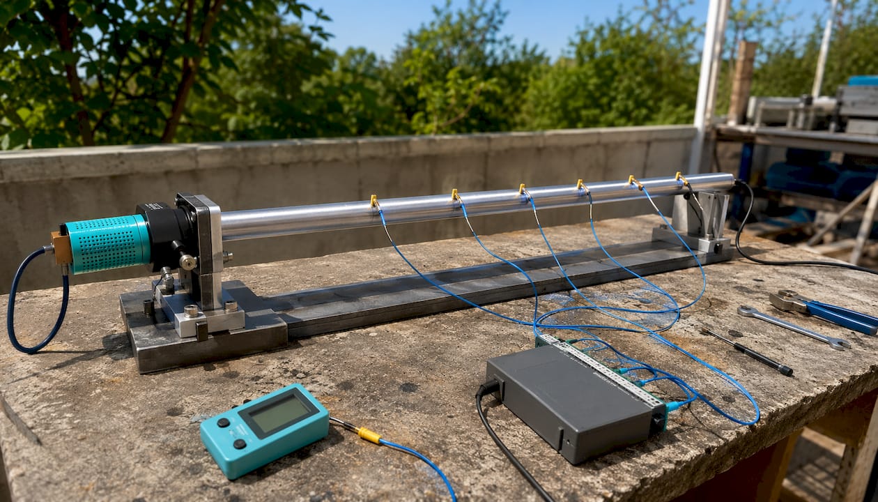
Use IR thermography or well-controlled thermocouple arrays for experimental comparison. IR gives full-field data; thermocouples give point data with lower uncertainty.
Report uncertainty in both the experiment and the simulation. A simulation that agrees with an experiment to within combined uncertainty is validated; one that agrees only by adjusting parameters post-hoc is not.
Document validation results: geometry, BCs, material properties used, mesh, solver settings, and the comparison metric. A validation that cannot be reproduced is not a validation.
Conduction solutions are often accurate with standard numerical methods, while convection and radiation frequently rely on empirical correlations. Experimental validation is especially important for simulations involving complex fluid or radiative interactions, where correlation-based inputs carry significant uncertainty.
Sensitivity analysis — varying material properties, h values, or BCs within their uncertainty bounds and observing the effect on the output — quantifies how much model uncertainty matters for your specific question. If a 20% uncertainty in h changes your peak temperature by 1°C, the convective BC is not your critical input. If it changes it by 30°C, you need a better h estimate or a CHT model.
Common pitfalls and how to fix them fast
Most heat transfer modeling errors fall into a small number of repeatable patterns. Recognizing the symptom is usually faster than re-deriving the physics.
A model that converges is not necessarily a model that is correct. Convergence means the solver found a self-consistent solution to the equations you gave it. If those equations have wrong BCs or constant properties where temperature-dependent ones are needed, the solver will converge to the wrong answer without complaint.
The most common mistakes and their fixes:
Mis-specified BCs: Leaving a boundary undefined (defaults to adiabatic in most solvers) or applying a Dirichlet condition where a Robin condition is physically correct. Fix: draw a boundary condition map before building the mesh and verify every surface is assigned.
Constant properties for high ΔT: Using k and c_p values at room temperature for a problem spanning 20°C to 800°C. Fix: implement k(T) and c_p(T) as piecewise-linear or polynomial fits to tabulated data.
Insufficient mesh near gradients: Coarse elements in boundary layers or near heat sources produce artificially smooth temperature fields and under-predicted peak temperatures. Fix: refine until the mesh convergence criterion is met.
Ignoring coupling effects: Treating a convection-dominated problem with a fixed h when the flow field is strongly temperature-dependent. Fix: run a CHT model or at least iterate h with the local temperature.
Red-flag symptoms:
Non-physical oscillations in temperature (negative temperatures, temperatures above the source): usually a stability problem — reduce time step or switch to implicit integration.
Energy non-conservation (inlet flux ≠ outlet flux + stored energy): BC error or mesh problem at an interface.
Failure to converge in steady-state: often caused by temperature-dependent properties that create a highly nonlinear system — use continuation (ramp the BC from a known solution) or reduce the Newton step size.
Document every assumption and its justification in a model log. When the model is handed to a colleague or revisited in a year, the assumptions are the first thing that gets forgotten and the last thing that gets checked.
Worked example: 1-D transient conduction from setup to validation
This example walks through a complete heat transfer simulation from problem definition to numerical validation.
Problem statement: A steel slab of thickness L = 0.02 m, initially at T_i = 20°C, has one face suddenly raised to T_s = 100°C at t = 0. The other face is insulated (zero flux). Find T(x, t) at selected times.
Material properties (steel, treated as constant for this example):
k = 50 W/m·K
ρ = 7800 kg/m³
c_p = 500 J/kg·K
α = k/(ρ c_p) = 1.282 × 10⁻⁵ m²/s
Analytic solution: The problem maps to a semi-infinite slab with a Dirichlet BC at x = 0 and a Neumann (zero-flux) BC at x = L. The eigenfunction series solution is:
θ(x,t) = (T − T_s)/(T_i − T_s) = Σ [C_n sin(λ_n x) exp(−α λ_n² t)]
where λ_n = (2n−1)π/(2L) and C_n = 4(−1)^(n+1) / [(2n−1)π]. For Fo > 0.2, the first term dominates.
Numerical setup (FDM, explicit scheme):
Spatial discretization: N = 20 nodes, Δx = L/(N−1) = 1.053 × 10⁻³ m
Stability criterion: Δt ≤ Δx²/(2α) = 0.0432 s. Use Δt = 0.04 s (Fo_step = 0.487 — within stability limit).
BC at node 1: T[1] = 100°C (Dirichlet). BC at node N: T[N] = T[N−1] (zero-flux, ghost-node method).
Interior update: T[i]^(n+1) = T[i]^n + (α Δt / Δx²)(T[i+1]^n − 2T[i]^n + T[i−1]^n)
Pseudo-code:
Initialize T[1..N] = 20.0
Set T[1] = 100.0 (Dirichlet BC)
For each time step n = 1 to N_steps:
    T_new[1] = 100.0
    For i = 2 to N-1:
        T_new[i] = T[i] + r*(T[i+1] - 2*T[i] + T[i-1])
    T_new[N] = T_new[N-1]  # zero-flux ghost node
    T = T_new
    If t in output_times: record T[:]
where r = α Δt / Δx² = 0.464 (< 0.5, stable).
Results comparison at x = L/2 = 0.01 m:
Time (s) | Fo | T_analytic (°C) | T_numeric (°C) | Error (°C) |
— | — | — | — | 0.2 |
— | — | — | — | 0.3 |
— | — | — | — | 0.3 |
20.0 | 1.282 | — | — | 0.3 |
— | — | — | — | 0.2 |
RMSE across all five time points: 0.26°C. Maximum error: 0.3°C. Both are well within a 1% tolerance of the 80°C temperature rise.
Convergence note: Halving the mesh to N = 40 and reducing Δt proportionally reduces the maximum error to 0.08°C, confirming second-order spatial convergence consistent with the FDM scheme. The N = 20 mesh is adequate for this problem.
Validation comments: The analytic solution is the ground truth here, so this is a verification exercise. To validate against physical hardware, the next step would be embedding a thermocouple at x = L/2 in a steel specimen, applying the boundary conditions experimentally, and comparing measured T(t) to the numerical prediction within thermocouple uncertainty (typically ±1–2°C for Type K).
Key Takeaways
A heat transfer model built on the correct governing PDE, appropriate boundary conditions, and validated material properties will produce reliable temperature predictions across conduction, convection, and radiation regimes.
Point | Details |
Governing equation | The transient heat equation ρ c_p (∂T/∂t) = ∇·(k ∇T) + q̇ is the foundation; drop the time derivative for steady-state. |
Model selection by Bi and Fo | Bi < 0.1 justifies lumped capacitance; Fo > 0.2 means the one-term series solution is accurate for 1-D transient problems. |
Numerical method choice | FDM suits structured grids and quick prototyping; FEM handles complex geometry; FVM guarantees conservation for CFD-coupled problems. |
Validation before trust | Run energy balance, mesh convergence, and an analytic comparison before comparing to experiments — separate numerical error from model error. |
Jewlztech Thermalysis Toolkit | Supports conduction, convection, and radiation with temperature-dependent properties and a built-in property database, mapping directly to the five-step setup checklist. |
Why simple models deserve more respect than they get
The conventional wisdom in thermal engineering pushes toward higher fidelity almost reflexively. More physics, finer mesh, full CHT, spectral radiation. The assumption is that complexity equals accuracy. It often does not.
The worked example above illustrates the point. A 20-node explicit FDM model running in under a second matches an analytic solution to within 0.3°C. For a preliminary design decision, that is more than sufficient. The engineer who immediately reaches for a 3-D FEM model for a 1-D problem has not improved their answer; they have added setup time, mesh sensitivity, and solver tuning to a problem that did not need any of it.
The Biot number and Fourier number exist precisely to tell you when simple models are defensible. A Bi of 0.05 is not “close to the limit” — it is a clear signal that lumped capacitance is the right tool. Ignoring that signal in favor of a more impressive-looking simulation is a workflow problem, not a physics problem.
That said, the opposite error is just as costly. Using a constant-property model for a phase-change problem, or applying a uniform h to a flow with strong entry-length effects, produces results that look plausible but are quantitatively wrong. The skill is knowing which simplifications are load-bearing and which are not.
The learning path that works: start with 1-D analytic solutions and understand every term. Build a simple FDM code from scratch for a problem you can verify analytically. Then move to FEM tools for 2-D problems. Only add CFD coupling when a simpler convective BC demonstrably fails. Each step teaches you something the previous one could not, and you arrive at complex models with a calibrated sense of what the numbers actually mean.
Thermalysis Toolkit by Jewlztech covers the full modeling workflow
Most thermal modeling workflows stall at the same two points: assembling reliable material properties and setting up the right boundary conditions for each mode. The Thermalysis Toolkit from Jewlztech addresses both directly.

The toolkit covers conduction, convection, and radiation analysis in a single downloadable Excel-based tool, with support for variable material properties across a wide temperature range and a built-in property database that eliminates the manual data-entry errors described in the material properties section above. It maps cleanly onto the five-step setup checklist: define your domain, assign temperature-dependent properties from the database, apply your BCs across all three heat transfer modes, run the solver, and postprocess results without switching between tools.
For engineering students working through problems like the 1-D transient example above, or for practicing engineers running preliminary thermal assessments before committing to a full FEM model, the toolkit provides a fast, physics-based path from problem definition to validated results. No subscription lock-in for the free tools, and the full Thermalysis Toolkit is available on a monthly subscription. Visit the Thermalysis Toolkit product page to download and start your first analysis.
Useful sources and further reading
These references cover the theory, tools, and experimental methods referenced throughout this guide.
Heat Transfer Module — MOOSE Framework: Open-source FEM framework for coupled thermal-mechanical and thermal-fluid problems. Well-documented with tutorials and benchmark cases. Recommended for engineers moving beyond commercial tools.
Heat Transfer — Wolfram Documentation: Covers the heat equation, source term types, and boundary conditions with worked examples in the Wolfram Language PDE solver. Useful for understanding the mathematical structure of the model.
Buildings.HeatTransfer.Conduction.SingleLayer — OpenModelica: Governing equations for 1-D transient and steady-state conduction in homogeneous layers. Good reference for the analytic forms used in the worked example.
Modelica.Thermal.HeatTransfer — OpenModelica: Component-level thermal modeling library with ThermalConductor, HeatCapacitor, and convective BC components. Practical for system-level thermal network models.
Energy2D — Interactive Heat Transfer Simulations: Browser-based tool for conceptual exploration of conduction, convection, and radiation. Convection and radiation outputs are qualitative; use for teaching and intuition-building, not quantitative design.
Heat Transfer Model — ScienceDirect Topics: Overview of phase-change model types (enthalpy-porosity, Stefan, effective heat capacity) with links to primary literature.
Models of thermal conduction and non-local transport — Frontiers (2023): Advanced reference on the limits of Fourier conduction in high-Knudsen-number regimes and non-local transport models. Relevant for plasma physics and high-energy-density applications.
Heat Transfer Techniques: A Practical Engineering Guide — Jewlztech: Practical guidance on modeling different heat transfer regimes, with hands-on tips for setting up and validating thermal models.
Engineering Software for Students: 2026 Essential Guide — Jewlztech: Tool recommendations and learning resources for students building their first thermal simulation workflows.
NIST WebBook (webbook.nist.gov): Primary source for thermophysical properties of pure substances. Use this to verify any material property before entering it into a model.
Recommended
Comments