
Heat Conduction Calculation: Formulas and Worked Examples

Updated: Sep 16
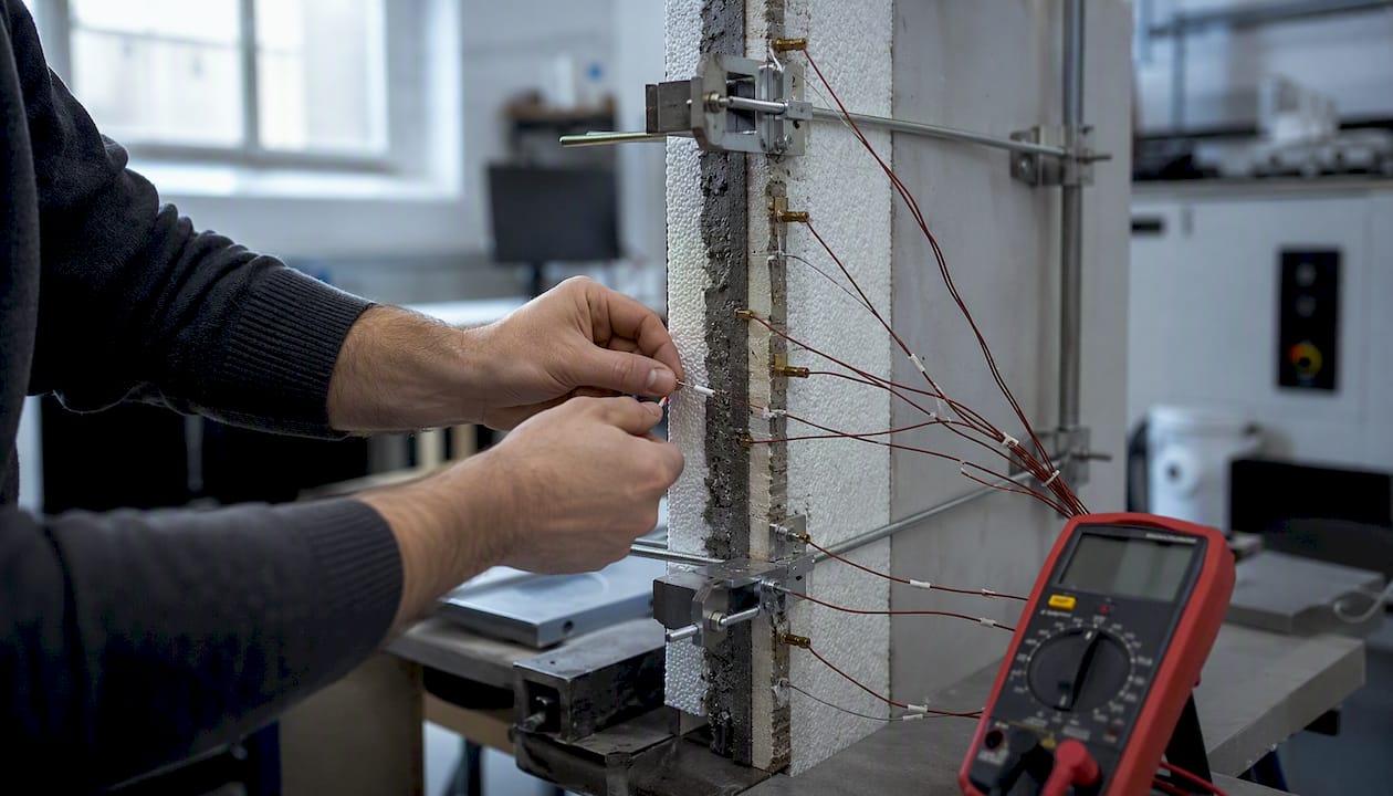
For most heat conduction calculations, you need one of two equations. For a flat slab at steady state: q = kA(T₁ − T₂)/L, where q is heat flow rate (W), k is thermal conductivity (W/m·K), A is cross-sectional area (m²), T₁ − T₂ is the temperature difference (K), and L is thickness (m). For the differential form, Fourier’s law of heat conduction states q = −kA dT/dx, where the negative sign confirms heat flows from hot to cold.
The one-line recipe for picking the right equation:
Plane slab, steady state: q = kA(T₁ − T₂)/L, or use thermal resistance R = L/(kA)
Composite wall (layers in series): R_total = R₁ + R₂ + … + Rₙ, then q = ΔT_total / R_total
Cylindrical geometry, steady state: Q̇ = 2πkℓ(T₁ − T₂) / ln(r₂/r₁), with R_cyl = ln(r₂/r₁) / (2πkℓ)
Transient problem: Check the Biot number first (Bi = hL/k); if Bi < 0.1, use lumped capacitance; otherwise solve the full heat diffusion equation
Complex geometry or variable k: Use numerical methods (FEM or FD) or a simulation tool
Key Takeaways
Steady-state heat conduction calculation starts with q = kA(T₁ − T₂)/L for a flat slab, builds to composite wall resistance networks using R = L/(kA), and escalates to numerical simulation when geometry or boundary conditions exceed analytic assumptions.
Point | Details |
Core slab formula | Use Q̇ = kA(T₁ − T₂)/L for 1D steady conduction; confirm units: (W/m·K)(m²)(K)/(m) = W. |
Composite wall method | Sum layer resistances R = L/(kA) in series; total heat rate is Q̇ = ΔT_total / R_total. |
Biot number rule | If Bi = hL/k < 0.1, lumped capacitance is valid; otherwise solve the full diffusion equation. |
Cylindrical geometry | Use R_cyl = ln(r₂/r₁)/(2πkℓ) for pipes and shells; do not apply the flat-slab formula to curved walls. |
Jewlztech Thermalysis Toolkit | Web-based engineering application for conduction, convection, radiation, and thermal resistance analysis with a built-in material property database. |
Table of Contents
What the symbols actually mean: heat flux, conductivity, resistance, and U-value
How 1D steady conduction works: from Fourier’s law to composite walls
Online calculators and software tools for quick verification
How engineers verify conduction calculations using simulation and benchmarking
When hand calculations are enough and when to reach for simulation
The Jewlztech Thermalysis Toolkit speeds up your conduction workflow
What the symbols actually mean: heat flux, conductivity, resistance, and U-value
Getting the physics right before plugging numbers in saves a lot of backtracking. Here is what each quantity represents and the units you need to keep consistent.
Heat transfer rate Q̇ (W) is the total power flowing through a surface. Heat flux q″ (W/m²) is that same power divided by area. In the slab formula above, q is often used loosely for Q̇ (total rate in watts), not the flux per unit area. Watch which convention a textbook or calculator uses.
Thermal conductivity k (W/m·K) describes how readily a material conducts heat. Metals have high k; insulating foams have low k. It depends on temperature, phase, and microstructure, so a single tabulated value is always an approximation. For most engineering calculations at moderate temperatures, treating k as constant is acceptable, but for wide temperature ranges you need to account for its variation.
Thermal resistance R (K/W) is the ratio of temperature difference to heat flow rate, exactly analogous to electrical resistance in Ohm’s law. A thicker slab or a smaller area increases R; a higher k decreases it. Thermal conductance U (W/K) is simply 1/R. In building science, the U-value is often expressed per unit area (W/m²·K), which is 1/(R_total × A). The MIT notes on heat transfer cover these definitions and their use in composite wall calculations in detail.
Symbol | Quantity | SI Unit | Common Alternative |
Q̇ | Heat transfer rate | W | BTU/hr |
q″ | Heat flux | W/m² | BTU/(hr·ft²) |
k | Thermal conductivity | W/(m·K) | BTU/(hr·ft·°F) |
R | Thermal resistance | K/W | °F·hr/BTU |
U | Thermal conductance (per area) | W/(m²·K) | BTU/(hr·ft²·°F) |
α | Thermal diffusivity | m²/s | ft²/hr |
L | Thickness | m | ft, in |
Where to find k values and how to convert units
A heat conduction calculation is only as good as the k value you feed it. The table below gives representative values at roughly room temperature to get you started.
Material | k (W/m·K) |
Copper | 0.22 |
Aluminum | 0.72 |
Carbon steel | ~50 |
Glass | 0.17 |
PMMA (acrylic) | 0.04 |
Polystyrene foam | 0.04 |
Air (still) | 0.013 |
These numbers shift with temperature. Copper’s k drops noticeably above 500°C; polystyrene’s rises slightly with temperature. For precision work, always pull values from a traceable database rather than a textbook appendix.
Unit conversion: 1 W/(m·K) = 0.5779 BTU/(hr·ft·°F). To go the other way, multiply BTU/(hr·ft·°F) by 1.731 to get W/(m·K).
Reliable sources for k values:
Wikipedia — Thermal conduction: Quick reference table covering metals, polymers, gases, and building materials
EngineeringToolbox: Searchable database with temperature-dependent values and unit toggles
Thermtest material database: Focused on measured thermal properties with instrument-specific data
NIST WebBook: Primary-source thermophysical data for gases and selected solids
As the University of Waterloo steady-state conduction notes caution, treating heat flow as purely one-dimensional is a simplification. If your geometry has significant transverse paths (corners, fins, fasteners), a single k lookup will not capture the full picture.
How 1D steady conduction works: from Fourier’s law to composite walls
Deriving the slab formula
Start with Fourier’s law in differential form: q = −kA dT/dx. For a homogeneous slab with constant k, constant A, and no internal heat generation, the temperature profile is linear. Integrating across thickness L from T₁ to T₂:
Q̇ = kA(T₁ − T₂) / L
Define thermal resistance as R = L/(kA). Then Q̇ = ΔT/R, which is the thermal Ohm’s law. This analogy is exact for steady-state conduction with no internal sources.
Building a composite wall resistance network
For a wall with n layers in series, resistances add directly:
Compute R_i = L_i / (k_i × A) for each layer
Sum them: R_total = R₁ + R₂ + … + Rₙ
Compute Q̇ = (T_hot − T_cold) / R_total
The U-value per unit area is U = 1 / (R_total × A)
Parallel heat paths (e.g., studs and insulation side by side) require a parallel resistance calculation instead: 1/R_parallel = 1/R_a + 1/R_b.
Pro Tip: When adding convective surface resistances (R_conv = 1/(hA)) at the boundaries, treat them as additional series resistors. The MIT heat transfer notes show this clearly for wall assemblies with interior and exterior film coefficients.
For a practical reference on steady-state conduction applications, the heat transfer techniques guide covers how these resistance networks feed into real design decisions.
When conduction is transient and how to handle it
Steady-state assumes temperatures are not changing with time. That assumption breaks down during startup, shutdown, or any time the boundary conditions shift faster than the material can equilibrate.
The governing equation for transient conduction is the heat diffusion equation:
∂T/∂t = α ∇²T + q̇_gen / (ρcₚ)
where α = k/(ρcₚ) is thermal diffusivity (m²/s), ρ is density (kg/m³), and cₚ is specific heat (J/kg·K). A high α means the material equilibrates quickly.
Deciding between lumped capacitance and the full equation
Compute the Biot number: Bi = hL_c / k, where h is the surface convection coefficient (W/m²·K) and L_c is a characteristic length (volume/surface area for a 3D body)
If Bi < 0.1, internal temperature gradients are small enough that the body can be treated as a single node. The lumped-capacitance criterion Bi < 0.1 is the standard rule of thumb
The lumped solution is: T(t) − T∞ = (T₀ − T∞) exp(−t / τ), where τ = ρcₚV / (hA_s) is the time constant
If Bi ≥ 0.1, you need either a series-solution (Heisler charts) or a numerical solver
Pro Tip: The thermal resistance analogy (R = L/(kA)) is strictly valid only for steady-state problems with no internal heat generation. Applying it to transient cases or systems with volumetric heat sources gives incorrect results. For those situations, the full diffusion equation is required — as the University of Waterloo notes make clear.
For problems that combine transient behavior with convection or radiation coupling, a heat transfer model that handles time-dependent boundary conditions is the practical path forward.
Online calculators and software tools for quick verification
No engineer should trust a hand calculation without at least one independent check. The tools below cover the range from quick sanity checks to full simulation.
Tool | Best for | Format |
Quick Q̇ = kAΔT/L checks, unit conversion | Interactive web calculator | |
Material k lookup, slab and pipe formulas | Web reference + calculator | |
Material property lookup, measured k data | Web database + calculator | |
MathWorks Simscape | Planar and cylindrical conduction blocks in system models | MATLAB/Simscape environment |
Jewlztech Thermalysis Toolkit | 1st order Heat transfer/Resistance Simulation encompassing different geometries | Web-based engineering application with built-in conduction analysis, material properties, thermal resistance modeling, and integrated heat-transfer calculations. |
The Thermalysis Toolkit provides a web-based engineering environment for performing heat-transfer calculations without requiring engineers to build and maintain their own calculation spreadsheets.
The MathWorks Simscape conductive heat transfer block implements both planar and cylindrical forms and exposes k, A, and thickness directly as inputs, making it straightforward to match against a hand calculation.
Step-by-step worked calculations with unit checks
Example 1: Single slab
Given: A 50 mm thick steel plate (k = 50 W/m·K), area A = 0.5 m², with T₁ = 200°C on one face and T₂ = 80°C on the other.
ΔT = 200 − 80 = 120 K
Q̇ = kA ΔT / L = 50 × 0.5 × 120 / 0.05
Q̇ = 60,000 W = 60 kW
Unit check: (W/m·K)(m²)(K)/(m) = W ✓
Sanity check: Steel conducts well; 60 kW across half a square meter with a 120 K drop is physically plausible. Run the same numbers in the HyperPhysics calculator to confirm.
Example 2: Composite wall
Given: A wall assembly with three layers (all A = 1 m²):
Layer 1: Brick, k₁ = 0.72 W/m·K, L₁ = 0.10 m
Layer 2: Fiberglass insulation, k₂ = 0.04 W/m·K, L₂ = 0.08 m
Layer 3: Gypsum board, k₃ = 0.17 W/m·K, L₃ = 0.013 m
Overall ΔT = 30 K (indoor to outdoor).
R₁ = 0.10 / (0.72 × 1) = 0.139 K/W
R₂ = 0.08 / (0.04 × 1) = 2.000 K/W
R₃ = 0.013 / (0.17 × 1) = 0.076 K/W
R_total = 0.139 + 2.000 + 0.076 = 2.215 K/W
Q̇ = 30 / 2.215 = 13.5 W
U-value = 1 / (R_total × A) = 1 / 2.215 = 0.45 W/m²·K
That is the expected result for a well-insulated wall assembly. The MIT notes derive this series-resistance approach in detail.
Example 3: Cylindrical pipe wall
Given: A steel pipe (k = 50 W/m·K), inner radius r₁ = 0.05 m, outer radius r₂ = 0.06 m, length ℓ = 2 m, T₁ = 150°C (inner), T₂ = 80°C (outer).
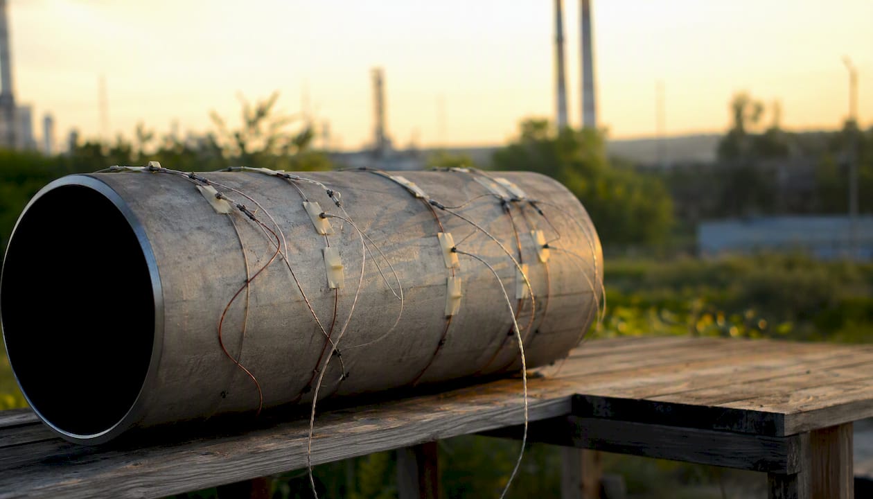
The cylindrical resistance formula is:
R_cyl = ln(r₂/r₁) / (2πkℓ)
ln(0.06/0.05) = ln(1.2) = 0.1823
R_cyl = 0.1823 / (2π × 50 × 2) = 0.1823 / 628.3 = 2.90 × 10⁻⁴ K/W
Q̇ = ΔT / R_cyl = 70 / 2.90 × 10⁻⁴ = 241,000 W ≈ 241 kW
Sanity check: A thin steel pipe wall with a 70 K drop conducts a large amount of heat because steel’s k is high and the wall is thin. For a pipe with insulation wrapped around it, add R_insulation = ln(r₃/r₂) / (2πk_ins × ℓ) in series. The MIT teaching notes on cylinders and spheres walk through this geometry in full.
For additional numeric examples across different geometries, the heat exchange examples guide is a useful companion.
Common mistakes and how to catch them before they cost you
Most errors in a heat conduction calculation fall into a short list of categories. Knowing them in advance is faster than debugging a result that looks wrong but you cannot explain why.
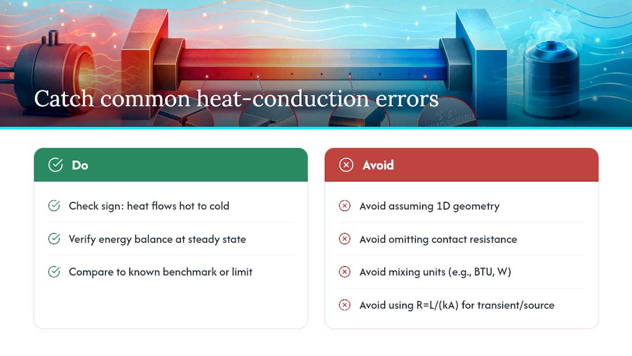
Wrong geometry assumption. Treating a corner, a fin, or a fastener path as purely 1D will underestimate heat loss. If significant transverse paths exist, the 1D result is a lower bound, not the answer. The University of Waterloo notes flag this explicitly: 1D simplification can underpredict total heat loss when multi-dimensional paths are present.
Forgetting contact resistance. At the interface between two materials, imperfect contact adds a resistance R_contact = 1/(h_c × A), where h_c is the contact conductance. This is easy to overlook and can dominate in bolted or pressed assemblies.
Using constant k across a wide temperature range. For most metals between 20°C and 200°C, constant k is a reasonable approximation.
Unit mismatch. Mixing BTU/hr and watts, or inches and meters, is the most common source of a result that is off by a factor of 3 to 10. Always write units next to every number during substitution and cancel them explicitly.
Applying the resistance analogy to transient or internally heated problems. R = L/(kA) is valid only for steady-state, no-source conditions. For systems with volumetric heat generation (q̇_gen ≠ 0) or time-varying temperatures, the full diffusion equation is required.
Pro Tip: Before finalizing any result, run three quick checks: (1) confirm the sign — heat flows from high to low temperature; (2) verify an energy balance — heat in equals heat out at steady state; (3) compare your answer to a known benchmark or a simpler limiting case. If your insulated wall conducts more heat than the same wall with no insulation, something is wrong.
How engineers verify conduction calculations using simulation and benchmarking
A hand calculation gives you a number. Verification gives you confidence that the number is right. The workflow most engineers follow:
Step 1 — Hand calculation: Derive the analytic result using the slab or cylindrical formula. Document every assumption: geometry, constant k, steady state, 1D, no internal generation.
Step 2 — Simple FEM model: Build a 2D or axisymmetric model in a FEM tool. Apply the same boundary conditions as the hand calc. Run a coarse mesh first.
Step 3 — Mesh refinement study: Halve the element size and rerun. If the heat flux changes by less than 5%, the mesh is adequate. If it changes more, refine further.
Step 4 — Boundary condition sensitivity: Perturb each boundary condition by ±10% and observe the effect on Q̇. This reveals which inputs drive the result and where measurement uncertainty matters most.
Step 5 — Experimental check (when available): Compare predicted surface temperatures or total heat rates against thermocouple or calorimeter data.
What to compare between hand calc and simulation: temperature profile shape (linear for 1D slab), heat flux magnitude at each surface, total heat rate Q̇, and dimensional convergence of the mesh.
The gap narrows when k is truly constant, geometry is genuinely 1D, and boundary conditions match exactly. Simulation platforms like MathWorks Simscape expose the same formula inputs as the hand calc, which makes side-by-side comparison straightforward.*
For engineers evaluating simulation tools beyond Simscape, the simulation alternatives guide covers practical options for verification workflows.
When hand calculations are enough and when to reach for simulation
Hand calculations are the right tool for preliminary sizing, homework, and design checks where geometry is simple and assumptions are clearly defensible. A composite wall U-value, a pipe insulation thickness, a quick Biot number check — these are exactly what the slab formula and resistance network are built for. They are fast, transparent, and easy to audit.
Simulation earns its place when geometry is genuinely complex (curved surfaces, fins, embedded heat sources), when k varies significantly with temperature, when transient coupling to convection or radiation matters, or when you need spatial temperature maps rather than a single Q̇ value. The Fourier’s law overview on ScienceDirect notes that many practical problems require transient analysis or coupled physics, and that is where analytic formulas reach their limit.
The most common mistake is skipping the hand calculation entirely and going straight to simulation. A simulation without a hand-calc anchor has no reference point. You cannot tell if a FEM result of 241 kW is reasonable unless you already know the analytic answer is in that range. Do both, in that order, every time.
Document your assumptions explicitly: steady or transient, 1D or 2D, constant or variable k, with or without contact resistance. A calculation that lists its assumptions is one that can be checked, revised, and trusted.
The Jewlztech Thermalysis Toolkit speeds up your conduction workflow
The Thermalysis Toolkit brings multiple heat-transfer calculations together in a single web-based engineering environment, allowing engineers to evaluate conduction, convection, radiation, and thermal resistance networks through an integrated interface.

The platform supports steady-state heat-transfer analysis using integrated conduction, convection, radiation, and thermal resistance calculations.
Sources
The sources below are the ones cited throughout this article. Each covers a specific part of the calculation workflow.
Recommended
Comments