
Forced Convection in Pipes: Correlations and Calculations

Updated: Aug 27

For fully developed laminar flow in a circular pipe, use Nu = 3.66 (constant wall temperature) or Nu = 4.36 (constant heat flux). For turbulent flow, the Dittus–Boelter equation.html) — Nu = 0.023 Re^0.8 Pr^n — covers Re within the typical range of fully developed turbulent flow, and Pr falls in the moderate to high thermal diffusivity fluids range, while the Gnielinski correlation gives better accuracy across moderate Reynolds and Prandtl numbers within its validity range. Pair either with f = 64/Re (laminar) or the Colebrook/Moody chart (turbulent) for pressure drop. One immediate caveat: a 2019 experimental study showed that the classical laminar constant Nu = 4.36 breaks down above Re ≈ 600–1000, where Nu begins rising with Re before transition. If your Richardson number exceeds 0.1, mixed convection is contaminating your results and none of these purely forced-convection correlations apply without correction.
Quick-reference formulae:
Laminar, fully developed, constant wall temperature: Nu = 3.66
Laminar, fully developed, constant heat flux: Nu = 4.36
Turbulent, Dittus–Boelter: Nu = 0.023 Re^0.8 Pr^n (n = 0.4 heating, n = 0.3 cooling)
Turbulent, Gnielinski: Nu = (f/8)(Re − 1000)Pr / [1 + 12.7(f/8)^0.5 (Pr^(2/3) − 1)], valid 3,000 ≤ Re ≤ 5×10^6
Sieder–Tate (large property variation): Nu = 0.027 Re^0.8 Pr^(1/3) (μ_b/μ_w)^0.14
Laminar friction factor: f = 64/Re
Turbulent friction factor: Colebrook equation or Moody chart; Haaland explicit approximation for quick computation
Pressure drop: ΔP = f (L/D) (ρV²/2) — Darcy–Weisbach
Regime limits: laminar Re below about 2,300; transitional Re range treated with caution; turbulent Re above approximately 10,000. Flag large property variation (viscosity ratio μ_b/μ_w far from 1) and check Ri = Gr/Re² before trusting any correlation.
Key Takeaways
The most reliable approach to forced convection in pipes is to select the correlation matched to your Re, Pr, and boundary condition, then bound the result with a two-correlation sensitivity check before committing to a design.
Point | Details |
Laminar Nu constants | Use Nu = 3.66 (CWT) or 4.36 (CHF) only when Re < 600–1000; above that, Nu rises with Re per 2019 experimental data. |
Turbulent default | Gnielinski is the preferred turbulent correlation (Re 3,000–5×10^6); Dittus–Boelter is acceptable for quick estimates above Re = 10,000. |
Friction and pressure drop | Use f = 64/Re for laminar; Colebrook or Haaland for turbulent; feed f into Gnielinski and Darcy–Weisbach for consistent h and ΔP. |
Mixed convection check | Compute Ri = Gr/Re² before trusting any forced-convection correlation; Ri > 0.1 invalidates purely forced-convection results. |
Jewlztech Thermalysis Toolkit | Runs Dittus–Boelter, Gnielinski, and Sieder–Tate correlations with built-in property evaluation and sensitivity sweeps in one web-based engineering analysis tool. |
Table of Contents
What dimensionless numbers govern forced convection in pipes?
How friction factor and pressure drop connect to heat transfer
Experimental pitfalls and what the 2019 data actually changed
Step-by-step worked example: heat transfer coefficient and pressure drop
Which correlation should you use for your specific situation?
Correction factors for non-circular pipes and annular geometries
What practitioners consistently get wrong about pipe heat transfer correlations
The Thermalysis Toolkit speeds up pipe heat-transfer calculations
What dimensionless numbers govern forced convection in pipes?
Forced convection is flow driven by an external device — a pump, fan, or compressor — rather than by buoyancy. That distinction matters because it defines which correlations apply and when buoyancy starts to corrupt your data.
Reynolds number: Re = ρVD_h/μ = VD_h/ν. This is the ratio of inertial to viscous forces and the primary regime indicator. Use the hydraulic diameter D_h = 4A_c/P for non-circular cross-sections, where A_c is cross-sectional area and P is wetted perimeter. For a circular pipe, D_h = D.
Prandtl number: Pr = μc_p/k = ν/α. It compares momentum diffusivity to thermal diffusivity. Liquid metals have Pr ≪ 1; water sits around 1–10 depending on temperature; oils can reach Pr > 1,000. Correlation validity ranges depend heavily on Pr, so check it before applying any formula.
Nusselt number: Nu = hD/k. It is the dimensionless convective heat transfer coefficient — the ratio of convective to conductive heat transfer across the fluid layer. Once you compute Nu from a correlation, recover h = Nu·k/D.
Grashof and Richardson numbers: Gr = gβΔTD³/ν². The Richardson number Ri = Gr/Re² compares buoyancy to inertial forces. When Ri > 0.1, buoyancy is no longer negligible and you are in mixed convection territory. The Metais and Eckert flow-regime map provides a graphical boundary between forced, mixed, and natural convection regimes as a function of Re, Gr, and Pr — useful for vertical pipe orientations especially.
Darcy–Weisbach: ΔP = f (L/D) (ρV²/2). This is the standard pressure-drop relation for pipe flow. The friction factor f is what links pressure drop to heat transfer in correlations like Gnielinski.
Property evaluation temperature: Always state where you evaluated fluid properties. The standard practice is to use the bulk mean temperature T_b = (T_in + T_out)/2 for most correlations. Sieder–Tate requires both bulk and wall temperatures. For large temperature differences, evaluate k, μ, and Pr at the film temperature T_f = (T_b + T_w)/2 to reduce error.
Pro Tip: Run a quick Ri check before any calculation. Compute Gr = gβΔTD³/ν² and divide by Re². If Ri > 0.1, switch to a mixed-convection reference or redesign the experiment to reduce ΔT or increase flow velocity.
Standard correlations for Nusselt number in pipe flow
The Nusselt number correlations used in practice fall into three regime groups: laminar fully developed, transitional (handle with care), and turbulent.
Laminar fully developed flow (Re < 2,300)
For a long pipe with a fully developed velocity and temperature profile, the Nusselt number is a constant — but which constant depends on the wall boundary condition.
Constant wall temperature (CWT): Nu = 3.66
Constant heat flux (CHF): Nu = 4.36
These are analytical results, not empirical fits. They hold when L/D is large enough that entrance effects are negligible (see Section 5 for entrance-length guidance). The CHF value is higher because a uniform heat flux creates a steeper near-wall temperature gradient than a uniform wall temperature does.
The 2019 experimental study mentioned in the opening is worth taking seriously here. Above that, Nu increases with Re even while friction stays at f = 64/Re — meaning the flow is still hydraulically laminar but thermally behaving differently than the classical solution predicts. If you are designing near the upper laminar range, use the revised correlations from that study rather than the textbook constant.
Dittus–Boelter (turbulent, Re > 10,000)
Nu = 0.023 Re^0.8 Pr^n
where n = 0.4 for heating (T_w > T_b) and n = 0.3 for cooling (T_w < T_b). Valid for Re within the typical range of fully developed turbulent flow, Pr falls in the moderate to high thermal diffusivity fluids range, and L/D ≥ 10. It assumes smooth tubes, negligible property variation, and fully developed flow.
Gnielinski correlation (turbulent, 3,000 ≤ Re ≤ 5×10^6)
Nu = (f/8)(Re − 1000)Pr / [1 + 12.7(f/8)^0.5 (Pr^(2/3) − 1)]
Valid for 0.5 ≤ Pr ≤ 2,000 and requires the Darcy friction factor f from Colebrook or Moody. Gnielinski is more accurate than Dittus–Boelter across a wider range, particularly at moderate Re (3,000–10,000) where Dittus–Boelter is not valid at all. The tradeoff is that you need f first, which adds a calculation step.
Sieder–Tate (large property variation)
Nu = 0.027 Re^0.8 Pr^(1/3) (μ_b/μ_w)^0.14
The viscosity-ratio correction factor (μ_b/μ_w)^0.14 accounts for the difference between bulk and wall viscosity. Use this when your fluid’s viscosity changes substantially across the pipe cross-section — oils and viscous polymers being the obvious cases. Evaluate μ_b at bulk temperature and μ_w at wall temperature. Without this correction, Dittus–Boelter can substantially mispredict h when viscosity gradients are steep.
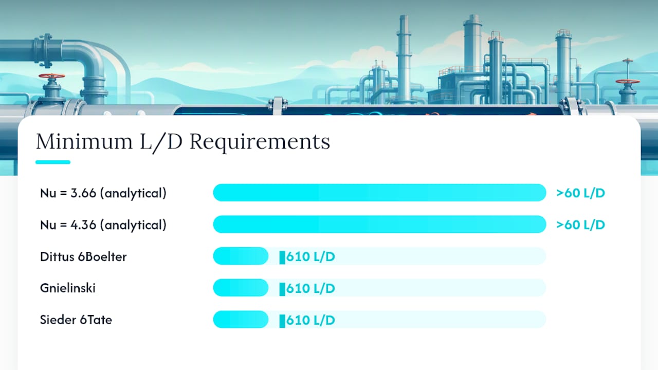
Correlation | Re range | Pr range | Boundary condition | Min L/D | Accuracy / notes |
Nu = 3.66 (analytical) | < 2,300 | Any | Constant wall temperature | > 60 | Exact for fully developed; breaks down near Re ≈ 600–1000 per 2019 data |
Nu = 4.36 (analytical) | < 2,300 | Any | Constant heat flux | > 60 | Same caveat above Re ≈ 600–1000 |
Dittus–Boelter | 10,000–5×10⁶ | 0.5–2,000 | Either (use correct n) | ≥ 10 | ±10%; avoid large ΔT or rough tubes |
Gnielinski | 3,000–5×10⁶ | 0.5–2,000 | Either | ≥ 10 | ±5–10%; requires f; preferred for moderate Re |
Sieder–Tate | 10,000–5×10⁶ | 0.5–2,000 | Either | ≥ 10 | Adds viscosity-ratio correction; use for oils or large ΔT |
How friction factor and pressure drop connect to heat transfer
The Darcy–Weisbach equation is the backbone of pipe pressure-drop calculations:
ΔP = f (L/D) (ρV²/2)
where f is the Darcy friction factor, L is pipe length, D is inner diameter, ρ is fluid density, and V is mean velocity. Getting f right is not optional — it feeds directly into Gnielinski and determines pumping power.
Laminar regime: f = 64/Re. No chart needed, no roughness correction. This holds as long as Re < 2,300 and the flow is fully developed.
Turbulent regime: f comes from the Colebrook–White equation:
1/√f = −2.0 log(ε/(3.7D) + 2.51/(Re√f))
This is implicit in f, which means you iterate or use an explicit approximation. The Moody chart is the graphical version — plot Re and relative roughness ε/D, read off f.
1/√f ≈ −1.8 log[(ε/(3.7D))^1.11 + 6.9/Re]
The Churchill equation is another fully explicit form that covers laminar, transitional, and turbulent regimes in a single expression — useful when you want a single formula in a spreadsheet or code.
Surface roughness effects: In laminar flow, roughness has essentially no effect on f or Nu — viscous forces dominate and the fluid does not “feel” the wall texture. In turbulent flow, relative roughness ε/D drives f upward once Re is high enough to push the flow into the fully rough regime. Higher f means higher ΔP and, through Gnielinski, a modestly higher Nu — but the ΔP penalty typically outweighs the heat-transfer gain. For heat exchangers, smooth tubes are almost always preferred unless surface features are intentionally engineered (twisted tape inserts, corrugated walls).
Worked pressure-drop example:
For gases at high velocity or long pipe runs, compressibility corrections apply when the Mach number exceeds roughly 0.3. Below that threshold, incompressible Darcy–Weisbach is accurate enough for most engineering purposes.
For Gnielinski, use the same f value you computed for ΔP — no separate friction calculation needed.
When roughness is unknown, assume hydraulically smooth (ε ≈ 0) for a conservative lower bound on f.
Always check whether your f is Darcy (f_D) or Fanning (f_F = f_D/4) — mixing them up introduces a factor-of-4 error in ΔP.
How entrance length changes your Nusselt number calculation
Fully developed correlations assume the velocity and temperature profiles have both reached their asymptotic shapes. That takes distance. Using a fully developed Nu in a short pipe or near an inlet will overestimate heat transfer resistance and underestimate h.
Hydrodynamic entrance length is the distance for the velocity profile to become fully developed:
Laminar: L_h ≈ 0.05 Re D
Turbulent: L_h ≈ 10–60 D (develops much faster due to turbulent mixing)
Thermal entrance length depends on both Re and Pr:
Laminar: L_t ≈ 0.05 Re Pr D (the Graetz problem)
Turbulent: L_t ≈ 10–60 D, similar to hydrodynamic but Pr-dependent
For water (Pr ≈ 5–7) in laminar flow at Re = 1,000, the thermal entrance length is roughly L_t ≈ 0.05 × 1,000 × 6 × D = 300D. That is a very long pipe before the temperature profile is fully developed. For air (Pr ≈ 0.71), L_t ≈ 35D at the same Re — much shorter.
In the entrance region, the local Nusselt number Nu_x is higher than the fully developed value because the thermal boundary layer is thin and the temperature gradient at the wall is steep. As x increases, Nu_x decays toward the asymptotic constant. The average Nusselt number over a length L is therefore always higher than the fully developed value, and the shorter the pipe, the larger that difference.
Pro Tip: When L/D < 60 in laminar flow, use the Hausen correlation for average Nu over the pipe length: Nu = 3.66 + 0.0668(D/L)Re·Pr / [1 + 0.04((D/L)Re·Pr)^(2/3)]. It accounts for the entrance region without requiring a local Nu integration.
Decision rule:
L/D ≥ 60 (laminar) or L/D ≥ 10 (turbulent): use fully developed correlations.
L/D < 60 (laminar): use an entry-region correlation (Hausen, Sieder–Tate with L/D correction, or local Nu integration).
L/D < 10 (turbulent): apply an entrance correction factor or use CFD.
Experimental pitfalls and what the 2019 data actually changed
Producing clean forced-convection pipe data is harder than it looks. The classical laminar constants (Nu = 3.66, 4.36) come from analytical solutions under idealized conditions — uniform properties, perfectly developed profiles, no buoyancy. Real experiments rarely satisfy all three simultaneously.
Buoyancy contamination is the most common problem. In vertical pipes with upward flow and wall heating, buoyancy aids the flow and increases Nu above the forced-convection value. In downward flow with heating, it opposes the flow and can trigger early transition. The Richardson number check (Ri = Gr/Re²) is the standard diagnostic — if Ri > 0.1, your data are mixed-convection data, not forced-convection data, regardless of how the experiment was labeled.
Heat flux control is the second major challenge. Achieving truly uniform heat flux along a pipe requires careful electrical heating design and good thermal insulation. Achieving constant wall temperature requires a secondary fluid with high thermal conductivity and flow rate — a condensing vapor or a well-stirred bath.
Instrumentation errors include thermocouple placement (surface vs. embedded), wall conduction along the pipe wall distorting local temperature readings, and small ΔT measurements where a 0.1°C thermocouple error represents a significant fraction of the total temperature difference.
The 2019 experimental study addressed these issues carefully — smooth circular tubes, vertical orientation, water, Re 400–6,000, constant heat fluxes 1–8 kW/m². Their key finding: the classical Nu = 4.36 holds only up to Re ≈ 600–1,000. Above that, Nu increases with Re while friction remains at f = 64/Re, meaning the flow is hydraulically laminar but thermally transitional. They developed revised laminar correlations and mapped transition boundaries. A 2024 arXiv literature review consolidates these and similar findings, highlighting that the transition region (Re ≈ 2,300–10,000) remains the least reliably covered by existing correlations.
Uncertainty checklist before trusting lab Nusselt numbers:
Compute Ri = Gr/Re² — if > 0.1, flag as mixed convection.
Confirm L/D is sufficient for the regime (≥ 60 laminar, ≥ 10 turbulent).
Verify thermocouple resolution relative to ΔT (aim for ΔT ≥ 10× thermocouple uncertainty).
Account for axial wall conduction — significant in thin-walled metal tubes with low-conductivity fluids.
Measure heat loss to surroundings and subtract from applied power before computing h.
Document the wall boundary condition (CWT or CHF) and the property evaluation temperature.
Pro Tip: Run the experiment at two or three different flow rates and check that Nu scales with Re as the correlation predicts. A flat Nu vs. Re curve in a supposedly turbulent regime is a strong sign of buoyancy contamination or premature transition.
Step-by-step worked example: heat transfer coefficient and pressure drop
Problem: Water flows through a smooth circular pipe, D = 0.02 m, L = 2.0 m. Inlet temperature T_in = 20°C, wall temperature T_w = 60°C (constant wall temperature). Find h and ΔP.
Step 1 — Film temperature and fluid properties:
T_f = (T_b + T_w)/2 ≈ (20 + 60)/2 = 40°C
At 40°C, water properties: ρ = 992 kg/m³, μ = 6.53×10⁻⁴ Pa·s, k = 0.631 W/(m·K), Pr = 4.34, c_p = 4179 J/(kg·K).
Step 2 — Compute Re:
Assume mean velocity V = 0.5 m/s.
Re = ρVD/μ = (992 × 0.5 × 0.02) / (6.53×10⁻⁴) ≈ 15,200
Re > 10,000 → turbulent. L/D = 2.0/0.02 = 100 ≥ 10 → fully developed correlations apply.
Step 3 — Select correlation and compute Nu:
Use Gnielinski (preferred for moderate Re). First, get f from Colebrook (smooth tube, ε/D ≈ 0):
f ≈ 0.316 Re^(−0.25) = 0.316 × (15,200)^(−0.25) ≈ 0.028 (Blasius approximation for smooth tubes, Re < 100,000)
Nu = (f/8)(Re − 1000)Pr / [1 + 12.7(f/8)^0.5(Pr^(2/3) − 1)] Nu = (0.028/8)(15,200 − 1,000)(4.34) / [1 + 12.7(0.028/8)^0.5(4.34^(2/3) − 1)] Nu = (0.0035)(14,200)(4.34) / [1 + 12.7 × 0.0591 × (2.63 − 1)] Nu = 215.9 / [1 + 12.7 × 0.0591 × 1.63] Nu = 215.9 / [1 + 1.224] = 215.9 / 2.224 ≈ 97.1
Step 4 — Compute h:
h = Nu × k / D = 97.1 × 0.631 / 0.02 ≈ 3,065 W/(m²·K)
Step 5 — Compute ΔP:
ΔP = f(L/D)(ρV²/2) = 0.028 × (2.0/0.02) × (992 × 0.5²/2) = 0.028 × 100 × 124 ≈ 347 Pa
Intermediate value | Result |
Film temperature T_f | 40°C |
Re | 15,200 |
Pr | 4.34 |
f (Blasius) | 0.028 |
Nu (Gnielinski) | 97.1 |
h | 3,065 W/(m²·K) |
ΔP | 347 Pa |
These sensitivities confirm that property evaluation temperature is the dominant uncertainty source in this calculation — consistent with the guidance in Section 2.
For a quick cross-check, the Dittus–Boelter equation gives Nu = 0.023 × (15,200)^0.8 × (4.34)^0.4 ≈ 88 — about 9% lower than Gnielinski. That spread (88 vs. 97) is a reasonable uncertainty bound for this calculation without experimental data.
Which correlation should you use for your specific situation?
The right answer depends on five things you should check in order: regime, boundary condition, L/D, property variation, and mixed convection risk.
Checklist:
Compute Re and Pr. Confirm which regime you are in (laminar < 2,300, transitional 2,300–10,000, turbulent > 10,000) and whether your Pr falls within the correlation’s valid range.
Identify your boundary condition. Constant wall temperature (CWT) or constant heat flux (CHF)? For laminar flow, this changes Nu by about 19%. For turbulent flow, the effect is smaller but still present in the Dittus–Boelter n exponent.
Check L/D. If L/D < 60 (laminar) or < 10 (turbulent), use an entrance-region correlation or apply a correction factor.
Assess property variation. If μ_b/μ_w deviates significantly from 1 (oils, high-ΔT cases), use Sieder–Tate or evaluate properties at film temperature.
Run the Ri check. Ri = Gr/Re² > 0.1 means mixed convection — stop and use a mixed-convection reference or reduce ΔT.
Flowchart decisions:
Fully developed laminar, Re < 600: use Nu = 3.66 (CWT) or 4.36 (CHF).
Laminar, Re 600–2,300: check the 2019 revised correlations; the classical constants underpredict Nu.
Transitional (2,300–10,000): no reliable single correlation. Use Gnielinski (it extends down to Re = 3,000) or interpolate with caution. Experimental data or CFD is the honest answer here.
Turbulent, smooth tube, moderate ΔT: Gnielinski is the default. Dittus–Boelter is acceptable for quick estimates when Re > 10,000.
Turbulent, large property variation: Sieder–Tate.
Turbulent, rough tube: use Colebrook f and feed it into Gnielinski.
Red flags that push you to experiment or CFD:
Ri > 0.1 (buoyancy not negligible)
Large ΔT causing viscosity to vary by more than 30–40% across the cross-section
Non-Newtonian fluid (see Section 9)
L/D < 5 with turbulent flow
Non-circular geometry without a reliable hydraulic-diameter correction (see Section 10)
Nanofluid or multiphase flow
Pro Tip: *Always run both Dittus–Boelter and Gnielinski for turbulent cases and use the spread as your uncertainty band.
Non-Newtonian fluids in forced convection within pipes
Standard pipe-flow correlations assume Newtonian behavior — shear stress proportional to shear rate, with a constant viscosity. Non-Newtonian fluids (polymer solutions, slurries, biological fluids, some nanofluids) violate this assumption, and applying Dittus–Boelter or Gnielinski directly to them produces unreliable results.
The most common model for non-Newtonian pipe flow is the power-law (Ostwald–de Waele) model: τ = K(du/dy)^n, where K is the consistency index and n is the flow behavior index. Shear-thinning fluids (n < 1, like most polymer solutions) have an effective viscosity that decreases toward the wall where shear rates are highest. Shear-thickening fluids (n > 1) behave oppositely.
For laminar flow of power-law fluids, a generalized Reynolds number Re_gen = ρV^(2−n)D^n / (K·8^(n−1)) replaces the standard Re. The Metzner–Reed correlation extends this framework to compute friction factors. For heat transfer, the Sieder–Tate structure is sometimes adapted with the generalized Re and a corrected Pr, but accuracy is limited and the validity ranges are narrower than for Newtonian fluids.
Turbulent non-Newtonian pipe flow is substantially more complex. Drag reduction (the Toms effect) in dilute polymer solutions can cut friction factors well below the Newtonian Colebrook prediction, and the corresponding heat transfer reduction follows — but not proportionally. For these cases, empirical correlations specific to the fluid class are necessary, and CFD with an appropriate rheological model is often the only reliable path for design-level accuracy.
The practical takeaway: if your fluid is non-Newtonian, identify the rheological model first, compute a generalized Re, and search for correlations developed specifically for that fluid class. Do not apply standard Newtonian correlations and expect better than order-of-magnitude accuracy.
Correction factors for non-circular pipes and annular geometries
The hydraulic diameter D_h = 4A_c/P is the standard way to extend circular-pipe correlations to non-circular geometries. For an annulus with inner radius r_i and outer radius r_o, D_h = 2(r_o − r_i). For a rectangular duct of sides a and b, D_h = 2ab/(a+b).

The agreement degrades for extreme geometries (very flat rectangles, thin annuli) because the velocity and temperature profiles in corners and narrow gaps differ fundamentally from the circular-pipe solution.
For laminar flow, the hydraulic-diameter substitution is less reliable. The fully developed Nu for a rectangular duct depends on aspect ratio: it ranges from Nu ≈ 7.54 (constant heat flux, square duct) down to Nu ≈ 5.39 for a 2:1 rectangle, compared to 4.36 for a circular pipe under the same boundary condition. Shah and London’s Laminar Flow Forced Convection in Ducts (1978) tabulates these values for a wide range of duct shapes and is the standard reference for non-circular laminar heat transfer.
For annular geometries, the heated surface matters. If only the inner wall is heated, Nu differs from the case where only the outer wall is heated — and both differ from the case of simultaneous heating. Kays and Crawford’s Convective Heat and Mass Transfer provides the relevant analytical solutions and tabulated correction factors for annuli.
For heat exchanger design, where annular and rectangular passages are common, these corrections are not optional.
Numerical methods for modeling forced convection in pipes
Empirical correlations give you a single number — an average Nu or a bulk h. Numerical methods give you the full spatial distribution of temperature, velocity, and heat flux, which matters when geometry is complex, boundary conditions vary along the pipe, or you need to resolve entrance effects and local hot spots.
Finite difference and finite volume methods are the workhorses of pipe-flow simulation. The governing equations — continuity, Navier–Stokes, and energy — are discretized on a computational grid. For axisymmetric laminar pipe flow, a 2D grid in the r–z plane is sufficient and computationally inexpensive. Turbulent flow requires either a fine near-wall mesh (direct numerical simulation or low-Re turbulence models) or wall functions to bridge the viscous sublayer.
Turbulence modeling is the central challenge in CFD for forced convection. The k–ε model (standard and realizable variants) is widely used for fully turbulent pipe flow and gives reasonable Nu predictions for smooth tubes. The k–ω SST model performs better in adverse pressure gradients and near-wall regions. For high-accuracy work — validating a new correlation or resolving transition — large eddy simulation (LES) or direct numerical simulation (DNS) is necessary but computationally expensive.
Conjugate heat transfer simulations couple the fluid domain to the solid pipe wall, capturing axial conduction in the wall and the effect of wall thermal resistance. This is important for thin-walled tubes with high-conductivity materials or for cases where the wall temperature is not uniform — both situations where the simple CWT or CHF boundary condition is an approximation.
Practical workflow: Start with a correlation to get a ballpark h and ΔP. Use those numbers to size the geometry and set boundary conditions for a CFD run. Validate the CFD against the correlation in a simple geometry (straight smooth pipe) before adding complexity. A heat transfer modeling guide can help bridge the gap between correlation-based estimates and full simulation.
For most engineering students and practitioners, the right sequence is: correlation → sensitivity sweep → CFD for complex geometry or validation. Jumping straight to CFD without a correlation baseline is a common mistake — you lose the sanity check that tells you whether your simulation result is in the right ballpark.
What practitioners consistently get wrong about pipe heat transfer correlations
The gap between what correlations promise and what they deliver in practice is wider than most textbooks admit. After working through the governing equations, validity ranges, and experimental caveats in this article, a few patterns stand out as persistently underappreciated.
The boundary condition is almost always treated as a detail rather than a fundamental input. In a real heat exchanger, neither constant wall temperature nor constant heat flux is exactly satisfied — the wall temperature varies along the length as the fluid heats up, and the local heat flux depends on the temperature difference between the two streams. The fix is not complicated: identify which idealization is closer to your actual condition and use it consistently.
The transitional regime (Re 2,300–10,000) gets far less attention than it deserves, partly because the textbook answer is “avoid it.” But many real systems — low-flow heat exchangers, building HVAC coils, medical device cooling loops — operate exactly there. The 2019 experimental data and the 2024 arXiv review both point to the same conclusion: existing correlations in this range carry large uncertainty, and the safe engineering response is to either design out of the transitional regime or validate with experiments specific to your geometry and fluid.
Sensitivity sweeps are underused. Computing Nu from a single correlation at nominal conditions and calling it done misses the point. Property variation, surface roughness, and entrance effects each contribute uncertainty. That band is what you actually need for a conservative design.
The Thermalysis Toolkit speeds up pipe heat-transfer calculations
Running the correlation sequence — Re, Pr, f, Nu, h, ΔP, Ri check, sensitivity sweep — manually for every design iteration is slow and error-prone. Jewlztech’s Thermalysis Toolkit integrates Dittus–Boelter, Gnielinski, and Sieder–Tate correlations in a single web-based engineering analysis environment with a built-in fluid property database, film-temperature evaluation, and batch sensitivity runs.

Where the toolkit earns its keep is in the sensitivity sweep. Change the inlet temperature, wall condition, or pipe diameter, and the property database updates automatically — no manual look-up, no risk of evaluating viscosity at the wrong temperature. The paired ΔP calculation uses the same f value feeding Gnielinski, so your heat-transfer and pressure-drop results stay consistent. For students working through heat transfer techniques or engineers validating a design before committing to CFD, that consistency check alone saves hours. Access the Thermalysis Toolkit at the product page and start with the free features to verify your correlation workflow before upgrading to the full library.
Sources
The sources below are the primary references used in this article. Consult the original papers for experimental datasets and the textbooks for derivations and extended correlation tables.
For reproducible calculations across all correlations covered here, the Jewlztech Thermalysis Toolkit implements the full correlation library with property databases — a practical complement to any of these references.
Recommended
Comments